![]()
Combining Multivariate Time Series and Derivatives Analytics
Python for Quant Finance Meetup, 15.02.2016
Dr. Yves J. Hilpisch
The Python Quants GmbH
About Me
![]()
![]()
For the curious:
- http://tpq.io (company Web site)
- http://pqp.io (Quant Platform)
- http://datapark.io (data science in the browser)
- http://fpq.io (For Python Quants conference)
- http://meetup.com/Python-for-Quant-Finance-London/ (1,200+ members)
- http://pff.tpq.io | http://dawp.tpq.io | http://lvvd.tpq.io
- http://hilpisch.com (all my talks and more)
- http://twitter.com/dyjh (events, talks, finance news)
Multivariate Vector Auto Regression with R
Processing the Data with Python
As an illustrative example we are going to analyze index data for the EURO STOXX 50 stock index and its volatility index VSTOXX. First, some Python imports.
import numpy as np
import pandas as pd
import seaborn as sns; sns.set()
%matplotlib inline
%load_ext rpy2.ipython
import warnings; warnings.simplefilter('ignore')
Second, some R imports.
%%R
library('zoo')
library('xts')
library('vars')
STOXX Limited provides open data for the two indicies on their Web site. We start with the VSTOXX data.
vs_url = 'http://www.stoxx.com/download/historical_values/h_vstoxx.txt'
vs = pd.read_csv(vs_url,  # filename
                 index_col=0,  # index column (dates)
                 parse_dates=True,  # parse date information
                 dayfirst=True, # day before month
                 header=2)  # header/column names
vs = vs.resample('MS') # resampling to month start frequency
A quick look at the most recent data rows.
vs.tail()
Retrieval of the EURO STOXX 50 data is a bit more involved.
cols = ['Date', 'SX5P', 'SX5E', 'SXXP', 'SXXE',
        'SXXF', 'SXXA', 'DK5F', 'DKXF', 'DEL']
es_url = 'http://www.stoxx.com/download/historical_values/hbrbcpe.txt'
es = pd.read_csv(es_url,  # filename
             header=None,  # ignore column names
             index_col=0,  # index column (dates)
             parse_dates=True,  # parse these dates
             dayfirst=True,  # format of dates
             skiprows=4,  # ignore these rows
             sep=';',  # data separator
             names=cols)  # use these column names
del es['DEL']
es = es.resample('MS')  # resampling to month start
Another quick look at this data set.
es.tail()
We write a sub-set of the data to disk as a CSV file.
data = vs.join(es)[['V2TX', 'SX5E']]
data.to_csv('SX5E_V2TX.csv')
A visualization of the data we are going to work with.
data.plot(subplots=True, color='b', figsize=(10, 6));

The time series are negatively correlated.
data.corr()
Vector Autoregregression
A VAR model is an $n$-equation, $n$-variable model in which each variable is explained by its own lagged values plus the current and past values of the remaining $n-1$ variables.
Assume we have an economic/financial system with a vector of (demeaned) variables $z_t$. The VAR in structural form is:
$$ Az_t = B_1z_{t-1} + B_2z_{t-2}+ ... + B_pz_{t-p}+u_t $$with
\begin{eqnarray*} Euu' = \Sigma_u = \begin{bmatrix} \sigma_{u1}^2 \ 0 \ \dots \ 0 \\ 0 \ \sigma_{u2}^2 \ \dots \ 0 \\ \vdots \ \vdots \ \ddots \ \vdots \\ 0 \ 0 \ \dots \ \sigma_{un}^2 \end{bmatrix} \end{eqnarray*}The model can also be written as:
$$ z_t = A_t^1B_1z_{t-1} + A_t^1B_2z_{t-2}+ ... + A_t^1B_pz_{t-p}+u_t $$In addition, it holds $E(u_t)=0$, $E(u_tu'_\tau)=\Sigma_u$ for $t=\tau$ and 0 otherwise.
VAR Modeling with R
The data can be read easily with R.
%%R
vd <- read.csv('SX5E_V2TX.csv')
data <- xts(vd[, -1], as.POSIXct(as.character(vd[,1]), format="%Y-%m-%d"))
Next, we generate a multivariate VAR model in R. We start with a simple one.
%%R
mod <- VAR(data,
      p=1,  # one lage only
      type='const');  # only mean relevant
The summary statistics from the model evaluation.
%%R
summary(mod)
Fitting of the EURO STOXX 50 index.
%R plot(mod, names='SX5E')

Forecast with the simple model.
%%R
pr = predict(mod, n.ahead=60, ci=0.9, dumvar = NULL)
plot(pr)

Second, a more sophisticated one.
%%R
mod <- VAR(data,
      p=12,  # using 12 lags
      season=12,  # seasonality of 12 lags
      type='both');  # both mean and trend
Fitting results (I).
%R plot(mod, names='SX5E')

Fitting results (II).
%R plot(mod, names='V2TX')

A forecast over 60 months.
%%R
pr = predict(mod, n.ahead=60, ci=0.9, dumvar = NULL)
plot(pr)

Model Calibration Data
Derivatives Model Calibration
Model calibration is a numerical optimization routine that looks for such parameters for a given model that best replicate market observed option quotes.
In our case, we fit a square-root diffusion (CIR) process with 3 parameters to options on the VSTOXX volatility index.
$$dv_t = \kappa (\theta - v_t) dt + \sigma \sqrt{v_t} dZ_t$$%run dx_srd_calibration.py
parameters.set_index('date').to_csv('srd_parameters.csv')
A possible calibration result might look as follows.
from IPython.display import Image
Image('calibration_result.png', width='75%')

The Data
We import the data set ...
para = pd.read_csv('srd_parameters.csv', index_col=0, parse_dates=True)
para[['initial_value', 'kappa', 'theta', 'sigma', 'MSE']].head()
... and plot it.
para[['initial_value', 'kappa', 'theta', 'sigma', 'MSE']].plot(
        figsize=(10, 12), subplots=True, color='b');

VAR Model for the Calibration Data
Setting up the VAR Model
We write the relevant sub-set of the data to disk ...
para = para[['initial_value', 'kappa', 'theta', 'sigma']]
para[para.index < '2014-3-1'].to_csv('srd_para_for_r.csv')
len(para[para.index >= '2014-3-1']) # out-of-sample period
... and read it with R.
%%R
vd <- read.csv('srd_para_for_r.csv')
data <- xts(vd[, -1], as.POSIXct(as.character(vd[, 1]), format="%Y-%m-%d"))
The VAR model based on the calibration data.
%R mod <- VAR(data, p=5, season=5, type='both');
For instance, theta shows a good fit.
%R plot(mod, names='theta')

Forecast for the Derivatives Model Parameters
We generate a forecast for 21 trading days.
%%R
pr = predict(mod, n.ahead=21, ci=0.75, dumvar = NULL)
plot(pr)

The forecast results are found in the fcst attribute.
%R attr(pr, 'names')
We pull the results to the Python run-time ...
%%R
ivs <- pr$fcst$initial_value
ks <- pr$fcst$kappa
ts <- pr$fcst$theta
ss <- pr$fcst$sigma
%Rpull ivs
%Rpull ks
%Rpull ts
%Rpull ss
... and store them in pandas DataFrame objects.
index = pd.date_range(start='2014-3-1', periods=len(ivs), freq='B')
fce = pd.DataFrame({'initial_value' : ivs[:, 0],
                  'kappa' : ks[:, 0],
                  'theta' : ts[:, 0],
                  'sigma' : ss[:, 0]}, index=index)
fce = fce.append(para[para.index == '2014-2-28']).sort()
fcl = pd.DataFrame({'initial_value' : ivs[:, 1],
                  'kappa' : ks[:, 1],
                  'theta' : ts[:, 1],
                  'sigma' : ss[:, 1]}, index=index)
fcl = fcl.append(para[para.index == '2014-2-28']).sort()
fcu = pd.DataFrame({'initial_value' : ivs[:, 2],
                  'kappa' : ks[:, 2],
                  'theta' : ts[:, 2],
                  'sigma' : ss[:, 2]}, index=index)
fcu = fcu.append(para[para.index == '2014-2-28']).sort()
The forecast results plotted with Python.
ax = fce.plot(figsize=(10, 12), subplots=True, style='b--');
fcl.plot(subplots=True, style='r--', ax=ax, label='lower', legend=False);
fcu.plot(subplots=True, style='y--', ax=ax, label='upper', legend=False);
para[['initial_value', 'kappa', 'sigma', 'theta']][
    para.index >= '2014-2-28'].plot(subplots=True,
                    style='b-', ax=ax, legend=False);

DX Analytics
Background and Philosophy
DX Analytics is a Python library for advanced financial and derivatives analytics authored and maintained by The Python Quants. It is particularly suited to model multi-risk and exotic derivatives and to do a consistent valuation of complex derivatives portfolios. It mainly uses Monte Carlo simulation since it is the only numerical method capable of valuing and risk managing complex, multi-risk derivatives books.
DX Analytics is open source, cf. http://dx-analytics.com & http://github.com/yhilpisch/dx.
The development of the library is guided by two central principles.
- global valuation approach: in practice, this approach translates into the non-redundant modeling of all risk factors (e.g. option underlyings like equity indexes) and the valuation of all derivative instruments by a unique, consistent numerical method — which is Monte Carlo simulation in the case of DX Analytics
- unlimited computing resources: in 2016, the technical infrastructures available to even smaller players in the financial industry have reached performance levels that 10 years ago seemed impossible or at least financially not feasible; in that sense "unlimited resources" is not to be understood literally but rather as the guiding principle that hardware and computing resources generally are no longer a bottleneck
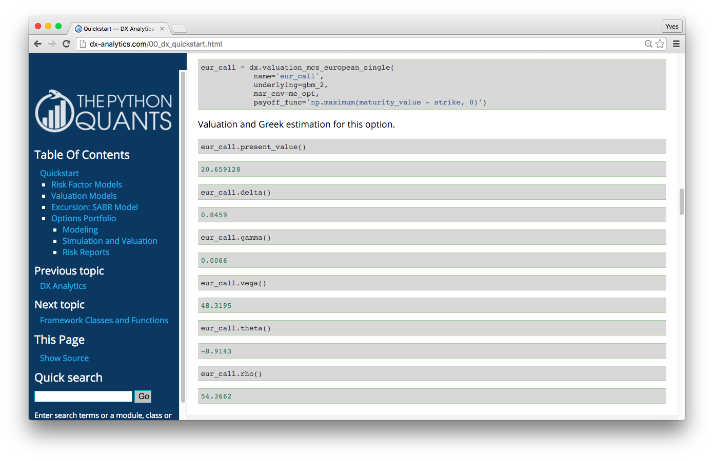
Example: DX Analytics — Quick Start
Example: DX Analytics — Complex
This example values a portfolio with 50 (correlated) risk factors and 250 options (European/American exercise) via Monte Carlo simulation in risk-neutral fashion with stochastic short rates.
http://dx-analytics.com/13_dx_quite_complex_portfolios.html
Modeling the VSTOXX Index
In what follows, we model the VSTOXX volatility index by a square-root diffusion process with DX Analytics. First, some imports.
import dx
import datetime as dt
import matplotlib.pyplot as plt
import seaborn as sns; sns.set()
All relevant data is stored in a market_environment object.
r = dx.constant_short_rate('r', 0.01)
me = dx.market_environment('me', para.index[0])
me.add_constant('initial_value', para['initial_value'].ix[0])
me.add_constant('kappa', para['kappa'].ix[0])
me.add_constant('theta', para['theta'].ix[0])
me.add_constant('volatility', para['sigma'].ix[0])
me.add_constant('final_date', dt.datetime(2014, 4, 18))
me.add_constant('currency', 'EUR')
me.add_constant('paths', 50000)
me.add_constant('frequency', 'W')
me.add_curve('discount_curve', r)
With this data, we instantiate the simulation object and simulate the process.
vstoxx = dx.square_root_diffusion('vstoxx', me)
paths = vstoxx.get_instrument_values()
The first 10 paths from the Monte Carlo simulation.
plt.figure(figsize=(10, 6));
plt.plot(vstoxx.time_grid, paths[:, :10]);
plt.gcf().autofmt_xdate();

A VSTOXX Option
We import options data for VSTOXX options and pick a particular option to do the further analyses.
h5 = pd.HDFStore('vstoxx_march_2014.h5', 'r')
od = h5['vstoxx_options']
od.set_index('DATE', drop=True, inplace=True)
h5.close()
strike = 19.0
odat = od[(od.TYPE == 'C')  # call option
        & (od.STRIKE == strike)  # fixed strike
        & (od.MATURITY == '2014-4-18')]  # fixed maturity date
The options price for the European call option over time.
odat['PRICE'].plot(figsize=(10, 6));

Modeling the VSTOXX Option
In a next step, we instantiate a valuation object for a single-risk derivative instrument — in our case a European call option.
me.add_constant('strike', strike)
me.add_constant('maturity', dt.datetime(2014, 4, 18))
payoff = 'np.maximum(maturity_value - strike, 0)'
call = dx.valuation_mcs_european_single(name='call', underlying=vstoxx,
        mar_env=me, payoff_func=payoff)
The valuation takes then only a single method call.
call.present_value()
We now take the calibration data and derive/re-calculate values for the option over the first quarter of 2014.
%%time
modvalues = []
for i in range(len(para)):
    pricing_date = para.index[i]
    initial_value, kappa, theta, sigma = para.ix[i][
        ['initial_value', 'kappa', 'theta', 'sigma']]
    vstoxx.update(pricing_date=pricing_date, initial_value=initial_value,
                  kappa=kappa, theta=theta, volatility=sigma)
    call.pricing_date = pricing_date
    modvalues.append(call.present_value())
The result is a time series with the call option values.
plt.figure(figsize=(10, 6));
plt.plot(odat.index, odat['PRICE'], label='market quote');
plt.plot(para.index, modvalues, '--', label='model value');
plt.ylabel('call value');
plt.legend(loc=0)
plt.gcf().autofmt_xdate();

Next, and maybe a bit more interesting, we do a option price forecast for April 2014 based on the VAR results.
%%time
collect = {}
for fc, name in zip([fce, fcl, fcu], ['mean', 'lower', 'upper']):
    values = [odat[odat.index == '2014-2-28']['PRICE']]
    for i in range(1, len(fc)):
        pricing_date = fc.index[i]
        initial_value, kappa, theta, sigma = fc.ix[i][
            ['initial_value', 'kappa', 'theta', 'sigma']]
        vstoxx.update(pricing_date=pricing_date, initial_value=initial_value,
                      kappa=kappa, theta=theta, volatility=sigma)
        call.pricing_date = pricing_date
        values.append(call.present_value())
    collect[name] = values
fcresults = pd.DataFrame(collect, fc.index)
The European call values based on the parameter forecasts visualized.
plt.figure(figsize=(10, 6));
plt.plot(odat.index, odat['PRICE'], label='market quote');
plt.plot(para.index, modvalues, '--', label='model value');
plt.plot(fcresults.index, fcresults['lower'], label='lower')
plt.plot(fcresults.index, fcresults['mean'], label='mean')
plt.plot(fcresults.index, fcresults['upper'], label='upper')
plt.ylabel('call value'); plt.legend(loc=0); plt.gcf().autofmt_xdate();

Summary
Some major insights from today:
- Python: Python is good at processing data, i.e. for data logistics
- Python & R: Python and R can easily interact with each other, exchanging data back and forth
- R: R provides powerful statistical libraries that might not be avalilable in Python
- VAR: multivariate vector auto regression can be efficiently and productively applied via the
varspackage (constant + trend + seasonality) - DX: DX Analytics is a Python library for advanced derivatives and risk analytics
- VAR + DX: we have combined mVAR with DX to generate forecasts of derivatives prices given a history of model parameters
![]()
http://tpq.io | @dyjh | team@tpq.io
Python Quant Platform | http://quant-platform.com
Python for Finance | Python for Finance @ O'Reilly
Derivatives Analytics with Python | Derivatives Analytics @ Wiley Finance
Listed Volatility and Variance Derivatives | Listed VV Derivatives @ Wiley Finance