![]()
Are Financial Markets Predictable?
— A Machine Learning Perspective
WORK IN PROGRESS
Dr Yves J Hilpisch
CEO The Python Quants | The AI Machine
Agenda
- Predictability Defined
- Why Does it Matter?
- Prediction Methods
- Correlation vs. Causation
- Finance History
- Efficient Markets
- Passive Investing
- Mathematics in Science
- Unreasonable Effectiveness of Data
- Artificial Intelligence
- ML-Based Applications
- Conclusions
Predictability Defined
Let $t=0$ denote the current point in time and let $t \in \{\ldots, -3, -2, -1, 0, 1, 2, 3, \ldots \}$ denote the relevant previous, current and future points in time.
Let $P_t$ denote the price of a financial instrument at time $t$. We have
$$P \in \{\ldots, P_{t=-2}, P_{t=-1}, P_{t=0}, P_{t=1}, \ldots \}$$or for short
$$P \in \{\ldots, P_{-2}, P_{-1}, P_{0}, P_{1}, \ldots \}.$$From Wikipedia (https://en.wikipedia.org/wiki/Markov_chain):
A Markov chain or Markov process is a stochastic model describing a sequence of possible events in which the probability of each event depends only on the state attained in the previous event.
- for a Markovian process, the distribution of price $P_t$ only depends on $P_{t-1}$
- for a non-Markovian process, the distribution of price $P_t$ can depend on the history of prices $P_{t-1}, P_{t-2}, P_{t-3}, \ldots$
To simplify things, let's assume that only the direction $d_t$ of the change in price at time $t$ is relevant.
$$d_t = \begin{cases}{} 1 \quad\textrm{if}\quad P_t - P_{t-1} > 0 \\ 0 \quad\textrm{if}\quad P_t - P_{t-1} \leq 0 \\ \end{cases}$$This gives the proces of directional changes $d \in \{\ldots, d_{-2}, d_{-1}, d_{0}, d_{1}, \ldots \}$. The problem we want to focus on, is whether we can predict the future directional change in price $d_1$ when we know the history of price changes $d_0, d_{-1}, d_{-2}, d_{-3}, \ldots$. Taking into account, say, five historical directional changes, a total of $2^5=32$ patterns can emerge.
from numpy.random import default_rng
rng = default_rng()
rng.integers(0, 2, 5)
array([1, 0, 1, 0, 0])
rng.integers(0, 2, 5)
array([1, 0, 0, 1, 0])
We are now interested in estimating — by whatever means — probabilities for $d_1 = 1$ and $d_1 = 0$ for any historical pattern $h = (d_0, d_{-1}, d_{-2}, d_{-3}, d_{-4})$.
Formally, the following conditional probabilities are of interest:
$$\begin{cases} \mathbf{P}(d_1=1|h)&=&p\\ \mathbf{P}(d_1=0|h)&=&1-p \end{cases}$$Such a problem is typically called a binary classification problem because, given a history $h$, one of two classes is to be picked — i.e., the one is to be picked for which a higher probability has been estimated. Classification is a special type of pattern recognition and also falls in the category of supervised learning algorithms in machine learning (ML).
From Wikipedia (https://en.wikipedia.org/wiki/Predictability):
Predictability is the degree to which a correct prediction or forecast of a system's state can be made either qualitatively or quantitatively.
From Google (https://developers.google.com/machine-learning/crash-course/classification/accuracy):
Accuracy is one metric for evaluating classification models. Informally, accuracy is the fraction of predictions our model got right.
Formally, we have for the accuracy:
$$\text{accuracy} = \frac{\text{# correct predictions}}{\text{# all predictions}}$$We say that a process of directional price changes is predictable if the accuracy of the predictions is significantly higher than 50%.
Why Does it Matter?
To be able to consistently well predict financial prices or directional changes in financial markets can be considered the holy grail in finance.
Why? Plain simple, because it would be a sure path to tremendous riches.
A simulation analysis with real-world data shall illustrate the point.
The following example is taken from chapter 14 of Hilpisch (2020): Artificial Intelligence in Finance, O'Reilly. First, some imports and the data preparation.
import random
import numpy as np
import pandas as pd
import cufflinks as cf
cf.set_config_file(offline=True, theme='ggplot')
url = 'https://hilpisch.com/aiif_eikon_eod_data.csv'
raw = pd.read_csv(url, index_col=0, parse_dates=True)
We pick the EUR/USD currency pair for the analysis with data for 2015 to 2019. bull stands for a long only strategy.
symbol = 'EUR='
raw['bull'] = np.log(raw[symbol] / raw[symbol].shift(1))
data = pd.DataFrame(raw['bull']).loc['2015-01-01':]
data.dropna(inplace=True)
In addition to the bull strategy, a random one, going long and short randomly, is generated. Also a bear strategy, going short only, is added.
rng = default_rng(100)
data['random'] = rng.choice([-1, 1], len(data)) * data['bull']
data['bear'] = -data['bull']
Assume now that a prediction model gets the top t percent of both the positive and negative movements (days) correct. Assume further, that for the rest it is not better than a random strategy. The following code creates the return series for such strategies.
def top(t):
    top = pd.DataFrame(data['bull'])
    top.columns = ['top']
    top = top.sort_values('top')
    n = int(len(data) * t)
    top['top'] = abs(top['top'])
    top['top'].iloc[n:-n] = rng.choice([-1, 1],
                len(top['top'].iloc[n:-n])) * top['top'].iloc[n:-n]
    data[f'{int(t * 100)}_top'] = top.sort_index()
for t in [0.1, 0.15]:
    top(t)
Assume now that the prediction model gets ratio percent of all directional movements correct and that it is not better than a random strategy for the rest.
def afi(ratio):
    correct = rng.binomial(1, ratio, len(data))
    random = rng.choice([-1, 1], len(data))
    strat = np.where(correct, abs(data['bull']), random * data['bull'])
    data[f'{int(ratio * 100)}_afi'] = strat
for ratio in [0.51, 0.6, 0.75, 0.9]:
    afi(ratio)
The following shows the first rows of the returns series of the different strategies.
print(data.head())
                bull    random      bear    10_top    15_top    51_afi  \
Date
2015-01-01  0.000413  0.000413 -0.000413  0.000413  0.000413  0.000413
2015-01-02 -0.008464 -0.008464  0.008464  0.008464  0.008464  0.008464
2015-01-05 -0.005767  0.005767  0.005767 -0.005767  0.005767  0.005767
2015-01-06 -0.003611 -0.003611  0.003611 -0.003611 -0.003611 -0.003611
2015-01-07 -0.004299  0.004299  0.004299  0.004299  0.004299  0.004299

              60_afi    75_afi    90_afi
Date
2015-01-01  0.000413  0.000413  0.000413
2015-01-02  0.008464  0.008464  0.008464
2015-01-05 -0.005767  0.005767  0.005767
2015-01-06  0.003611  0.003611 -0.003611
2015-01-07 -0.004299  0.004299  0.004299
This translates into the following gross performance values. Throughout, zero transaction costs are assumed.
data.sum().apply(np.exp)
bull       0.926676
random     1.245684
bear       1.079126
10_top    12.322428
15_top    23.343766
51_afi    18.627366
60_afi    16.950628
75_afi    43.611802
90_afi    90.892721
dtype: float64
This translates into the following gross performance values over time, again assuming zero transaction costs.
data.cumsum().apply(np.exp).iplot(colorscale='reds')
Prediction Methods
From Wikipedia (https://en.wikipedia.org/wiki/Stock_market_prediction):
Stock market prediction is the act of trying to determine the future value of a company stock or other financial instrument traded on an exchange. The successful prediction of a stock's future price could yield significant profit. The efficient-market hypothesis suggests that stock prices reflect all currently available information and any price changes that are not based on newly revealed information thus are inherently unpredictable. Others disagree and those with this viewpoint possess myriad methods and technologies which purportedly allow them to gain future price information.
Over time, financial practitioners have used a plethora of methods in their effort to predict financial markets:
- fundamental analysis (value/growth)
- technical analysis (trends, support, breakout)
- statistical methods (regression, Bayesian models)
- time series modeling (ARIMA, ARCH, GARCH)
- artificial intelligence (ML, DL, RL)
Technical analysis methods are still pretty popular and intuitively appealing. One of the most simple examples is the use of two simple moving averages (SMAs) to decide whether to go long or short a financial instrument.
data = pd.DataFrame(raw[symbol])
data['SMA1'] = data[symbol].rolling(42).mean()
data['SMA2'] = data[symbol].rolling(252).mean()
data['POSITION'] = np.where(data['SMA1'] > data['SMA2'], 1, -1)
The idea here is to go long when the shorter/faster SMA is above the longer/slower SMA and short otherwise.
data.iloc[252:].iplot(secondary_y='POSITION')
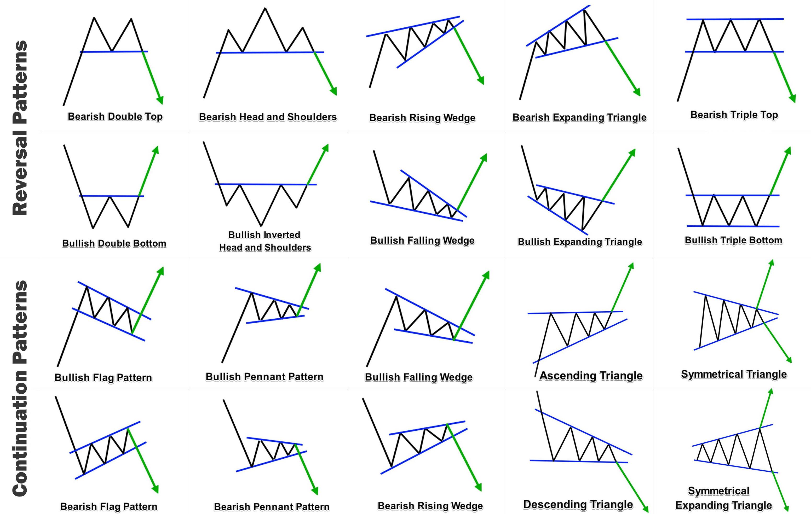
Other technical analysis methods are based on certain price formations — or more generally patterns in prices. Source reddit.
Correlation vs. Causation
Several stylized facts about financial markets show stable, non-zero correlations over time.
Take the case of the correlation between the S&P 500 (.SPX) and its volatility index VIX (.VIX) — (1).
data = raw[['.SPX', '.VIX']]
rets = np.log(data / data.shift(1)).dropna()
print(rets.corr())
          .SPX      .VIX
.SPX  1.000000 -0.809235
.VIX -0.809235  1.000000
Take the case of the correlation between the S&P 500 (.SPX) and its volatility index VIX (.VIX) — (2).
rets.iplot(kind='scatter', x='.SPX', y='.VIX', mode='markers',
           size=4, bestfit=True, xTitle='.SPX', yTitle='.VIX')
Take the case of the correlation between the S&P 500 (.SPX) and its volatility index VIX (.VIX) — (3).
rets['.SPX'].rolling(252).corr(rets['.VIX']).dropna().iplot(bestfit=True)
However, neither index is a leading indicator (cause) for the other — (1).
rets['.SPX'].corr(rets['.VIX'].shift(1))
0.013860922375245097
rets['.SPX'].rolling(252).corr(rets['.VIX'].shift(1)).dropna().iplot(bestfit=True)
However, neither index is a leading indicator (cause) for the other — (2).
rets['.VIX'].corr(rets['.SPX'].shift(1))
0.06536531043304598
rets['.VIX'].rolling(252).corr(rets['.SPX'].shift(1)).dropna().iplot(bestfit=True)
Finance History
Finance has gone through multiple phases and paradigm shifts over time (1):
- The ancient period (pre-1950): A period mainly characterized by informal reasoning, rules of thumb, and the experience of market practitioners. See Rubinstein (2006): A History of the Theory of Investments, Wiley Finance.
- The classical period (1950–1980): A period characterized by the introduction of formal reasoning and mathematics to the field. See Hilpisch (2021): Financial Theory with Python, O'Reilly.
- The modern period (1980–2000): This period generated many advances in specific subfields of finance (for example, computational finance) and tackled, among others, important empirical phenomena in the financial markets, such as stochastic interest rates or stochastic volatility. See Hilpisch (2015): Derivatives Analytics with Python, Wiley Finance.
Finance has gone through multiple phases and paradigm shifts over time (2):
- The computational period (2000–2020): This period saw a shift from a theoretical focus in finance to a computational one, driven by advances in both hardware and software used in finance. See Hilpisch (2018): Python for Finance, 2nd ed., O'Reilly.
- The artificial intelligence period (post-2020): Advances in artificial intelligence (AI) and related success stories have spurred interest to make use of the capabilities of AI in the financial domain. AI-first finance describes the shift from simple, in general linear, models in finance to the use of advanced models and algorithms from AI. See Hilpisch (2020): Artificial Intelligence in Finance, O'Reilly.
Efficient Markets
Eugene F. Fama (1965): "Random Walks in Stock Market Prices":
For many years, economists, statisticians, and teachers of finance have been interested in developing and testing models of stock price behavior. One important model that has evolved from this research is the theory of random walks. This theory casts serious doubt on many other methods for describing and predicting stock price behavior—methods that have considerable popularity outside the academic world. For example, we shall see later that, if the random-walk theory is an accurate description of reality, then the various "technical" or "chartist" procedures for predicting stock prices are completely without value.
Michael Jensen (1978): "Some Anomalous Evidence Regarding Market Efficiency":
A market is efficient with respect to an information set S if it is impossible to make economic profits by trading on the basis of information set S.
From Investopedia (see Forms of Market Efficiency):
- The weak form suggests today’s stock prices reflect all the data of past prices and that no form of technical analysis can aid investors.
- The semi-strong form submits that because public information is part of a stock's current price, investors cannot utilize either technical or fundamental analysis, though information not available to the public can help investors.
- The strong form version states that all information, public and not public, is completely accounted for in current stock prices, and no type of information can give an investor an advantage on the market.
John Hull (2012): Options, Futures, and Other Derivatives.
The Markov property of stock prices is consistent with the weak form of market efficiency. This states that the present price of a stock impounds all the information contained in a record of past prices. If the weak form of market efficiency were not true, technical analysts could make above-average returns by interpreting charts of the past history of stock prices. There is very little evidence that they are in fact able to do this.
If a stock price follows a (simple) random walk (no drift & normally distributed returns), then it rises and falls with the same probability of 50% ("toss of a coin").
In such a case, the best predictor of tomorrow’s stock price — in a least-squares sense — is today’s stock price.
A practical example based on OLS regression (1).
url = 'http://hilpisch.com/pyalgo_eikon_eod_data.csv'
raw = pd.read_csv(url, index_col=0, parse_dates=True).dropna()
raw.iloc[:5, :5]
| AAPL.O | MSFT.O | INTC.O | AMZN.O | GS.N | |
|---|---|---|---|---|---|
| Date | |||||
| 2010-01-04 | 30.572827 | 30.950 | 20.88 | 133.90 | 173.08 |
| 2010-01-05 | 30.625684 | 30.960 | 20.87 | 134.69 | 176.14 |
| 2010-01-06 | 30.138541 | 30.770 | 20.80 | 132.25 | 174.26 |
| 2010-01-07 | 30.082827 | 30.452 | 20.60 | 130.00 | 177.67 |
| 2010-01-08 | 30.282827 | 30.660 | 20.83 | 133.52 | 174.31 |
A practical example based on OLS regression (2).
raw['RANDOM'] = 100
raw['RANDOM'].iloc[1:] += np.random.standard_normal(len(raw) - 1).cumsum()
raw[['GS.N', 'RANDOM']].normalize().iplot();
A practical example based on OLS regression (3).
symbol = 'RANDOM'
symbol = 'GS.N'
data = pd.DataFrame(raw[symbol])
lags = 5
cols = list()
for lag in range(1, lags + 1):
    col = f'lag_{lag}'
    data[col] = data[symbol].shift(lag)
    cols.append(col)
data.dropna(inplace=True)
A practical example based on OLS regression (4).
reg = np.linalg.lstsq(data[cols], data[symbol], rcond=-1)[0]
reg
array([ 0.980752 , 0.03435725, -0.01860718, 0.00624259, -0.00272114])
Remark: The use of lagged prices violates a major assumption of OLS regression, namely that the independent variables be uncorrelated.
data[cols].corr()
| lag_1 | lag_2 | lag_3 | lag_4 | lag_5 | |
|---|---|---|---|---|---|
| lag_1 | 1.000000 | 0.997883 | 0.995849 | 0.993748 | 0.991664 |
| lag_2 | 0.997883 | 1.000000 | 0.997880 | 0.995847 | 0.993742 |
| lag_3 | 0.995849 | 0.997880 | 1.000000 | 0.997879 | 0.995844 |
| lag_4 | 0.993748 | 0.995847 | 0.997879 | 1.000000 | 0.997876 |
| lag_5 | 0.991664 | 0.993742 | 0.995844 | 0.997876 | 1.000000 |
Passive Investing & Index Funds
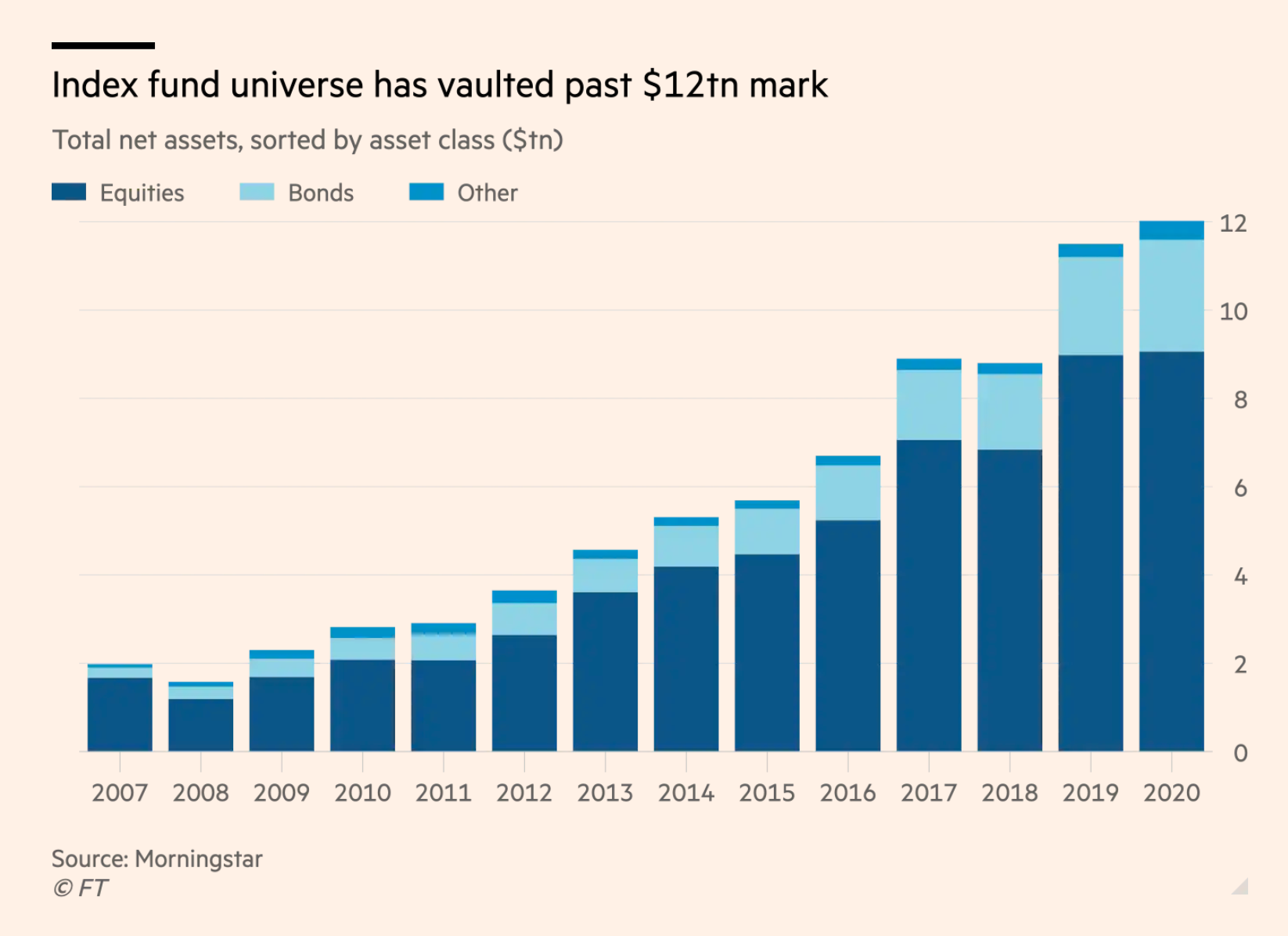
Robin Wigglesworth: "A theory of (almost) everything for financial markets." Financial Times, 29. December 2020.
It is true that the indices that passive funds track have over time morphed from being supposedly neutral snapshots of markets into something that actually exerts power over them, thanks to the growth of passive investing.
Mr Green argues that this helps explain why active managers are actually seeing their performance worsen as passive investing grows. The more money index funds garner, the better their holdings do in exact proportion to their weighting, and the harder it is for traditional discretionary investors to keep up.
Robin Wigglesworth: "A theory of (almost) everything for financial markets." Financial Times, 29. December 2020.
Mathematics in Science
Sabine Hossenfelder (2018): Lost in Math — How Beauty Leads Physics Astray.
They were so sure, they bet billions on it. For decades physists told us they kew where the next discoveries were waiting. ... The experiments didn't reveal anything new.
What failed physicists wasn't their math; it was their choice of math. They believed that Mother Nature was elegant, simple, and kind about providing clues. They thought they could hear her whisper when they were talking to themselves. Now Nature spoke, and she said nothing, loud and clear.
Eugene F. Fama and Kenneth R. French (2004): "The Capital Asset Pricing Model: Theory and Evidence."
The attraction of the CAPM is that it offers powerful and intuitively pleasing predictions about how to measure risk and the relation between expected return and risk. Unfortunately, the empirical record of the model is poor—poor enough to invalidate the way it is used in applications. The CAPM’s empirical problems may reflect theoretical failings, the result of many simplifying assumptions. But they may also be caused by difficulties in implementing valid tests of the model.
The version of the CAPM developed by Sharpe (1964) and Lintner (1965) has never been an empirical success. ... The problems are serious enough to invalidate most applications of the CAPM.
Unreasonable Effectiveness of Data
Alon Halevy et al. (2009): "The Unresonable Effectiveness of Data."
Eugene Wigner’s article "The Unreasonable Effectiveness of Mathematics in the Natural Sciences" examines why so much of physics can be neatly explained with simple mathematical formulas such as $f = ma$ or $e = mc^2$. Meanwhile, sciences that involve human beings rather than elementary particles have proven more resistant to elegant mathematics. Economists suffer from physics envy over their inability to neatly model human behavior. An informal, incomplete grammar of the English language runs over 1,700 pages. Perhaps when it comes to natural language processing and related fields, we’re doomed to complex theories that will never have the elegance of physics equations. But if that’s so, we should stop acting as if our goal is to author extremely elegant theories, and instead embrace complexity and make use of the best ally we have: the unreasonable effectiveness of data.
Artificial Intelligence
Big Financial Data + Artificial Intelligence = AI-First Finance.
ML-Based Applications
Assume that there are (persistent) patterns in financial markets that, when identified, allow to predict future price movements. To simplify things, assume binary features and labels only.
symbol = 'RANDOM'
symbol = 'GS.N'
def create_features(lags):
    data = pd.DataFrame(raw[symbol])
    data['r'] = np.log(data[symbol] / data[symbol].shift(1))
    data['d'] = np.sign(data['r'])
    data['d'] = data['d']
    cols = list()
    for lag in range(1, lags + 1):
        col = f'lag_{lag}'
        data[col] = data['d'].shift(lag)
        cols.append(col)
    data.dropna(inplace=True)
    data[['d'] + cols] = data[['d'] + cols].astype(int)
    return data, cols
We now have a simple classification problem for which we can train appropriate models through supervised learning.
lags = 2
data, cols = create_features(lags)
2 ** lags # number of patters
4
data.tail()
| GS.N | r | d | lag_1 | lag_2 | |
|---|---|---|---|---|---|
| Date | |||||
| 2019-12-24 | 229.91 | 0.003573 | 1 | 1 | -1 |
| 2019-12-26 | 231.21 | 0.005638 | 1 | 1 | 1 |
| 2019-12-27 | 230.66 | -0.002382 | -1 | 1 | 1 |
| 2019-12-30 | 229.80 | -0.003735 | -1 | -1 | 1 |
| 2019-12-31 | 229.93 | 0.000566 | 1 | -1 | -1 |
Let's divide the data into training and testing data.
split = int(0.8 * len(data))
train = data.iloc[:split]
test = data.iloc[split:]
One can simply use a frequentist approach to the prediction problem (1).
import copy
sel = copy.deepcopy(cols)
sel.append('d')
grouped = train.groupby(sel)
res = grouped['d'].size().unstack(fill_value=0)
# relative freuency for upward movement
res['perc'] = res[1] / res.sum(axis=1)
One can simply use a frequentist approach to the prediction problem (2).
res # perc = relative freuency for upward movement
| d | -1 | 0 | 1 | perc | |
|---|---|---|---|---|---|
| lag_1 | lag_2 | ||||
| -1 | -1 | 212 | 0 | 237 | 0.527840 |
| 1 | 237 | 0 | 283 | 0.544231 | |
| 0 | 1 | 0 | 0 | 2 | 1.000000 |
| 1 | -1 | 262 | 1 | 257 | 0.494231 |
| 0 | 1 | 0 | 1 | 0.500000 | |
| 1 | 257 | 1 | 259 | 0.500967 |
Let's use more lags and thereby more patterns.
lags = 5
data, cols = create_features(lags)
2 ** lags # number of patters
32
train = data.iloc[:split]
test = data.iloc[split:]
Any classifier can be applied to learn about patterns with predictive power (1).
from sklearn.tree import DecisionTreeClassifier
from sklearn.metrics import accuracy_score
model = DecisionTreeClassifier(max_depth=3)
model.fit(train[cols], train['d'])
DecisionTreeClassifier(max_depth=3)
accuracy_score(train['d'], model.predict(train[cols])) # in-sample
0.554228855721393
accuracy_score(test['d'], model.predict(test[cols])) # out-of-sample
0.48
Any classifier can be applied to learn about patterns with predictive power (2).
from sklearn.svm import SVC
model = SVC()
model.fit(train[cols], train['d'])
SVC()
accuracy_score(train['d'], model.predict(train[cols])) # in-sample
0.5681592039800994
accuracy_score(test['d'], model.predict(test[cols])) # out-of-sample
0.478
Any classifier can be applied to learn about patterns with predictive power (3).
from sklearn.neural_network import MLPClassifier
model = MLPClassifier(shuffle=False)
model.fit(train[cols], train['d'])
MLPClassifier(shuffle=False)
accuracy_score(train['d'], model.predict(train[cols])) # in-sample
0.5502487562189055
accuracy_score(test['d'], model.predict(test[cols])) # out-of-sample
0.462
Conclusions
Let's summarize:
- Being able to predict financial markets/prices is the holy grail in finance — it is a sure path to immense riches.
- Financial practitioners and academics have tried many different methods in the past to predict financial markets/prices.
- While there seem to be a number of persistent correlations in the markets, causal relationships are hard to identify or exploit.
- The Efficient Market Hypothesis has seen strong empirical support in the past; the EMH basically says that market are not predictable.
- While mathematics and normative ideas dominated finance in the past, finance has become a data-driven discipline with many emerging AI applications.
- AI/ML/DL might open a path to identify and exploit statistical and economical inefficiencies in financial markets.