Derivatives Analytics with Python
Dr. Yves J. Hilpisch
The Python Quants GmbH
O'Reilly Webcast – 24. June 2014
The Python Quant
- Founder and MD of The Python Quants GmbH
- Lecturer Mathematical Finance at Saarland University
- Co-organizer of "For Python Quants" conference in New York
- Organizer of "Python for Quant Finance" meetup in London
- Organizer of "Python for Big Data Analytics" meetup in Berlin
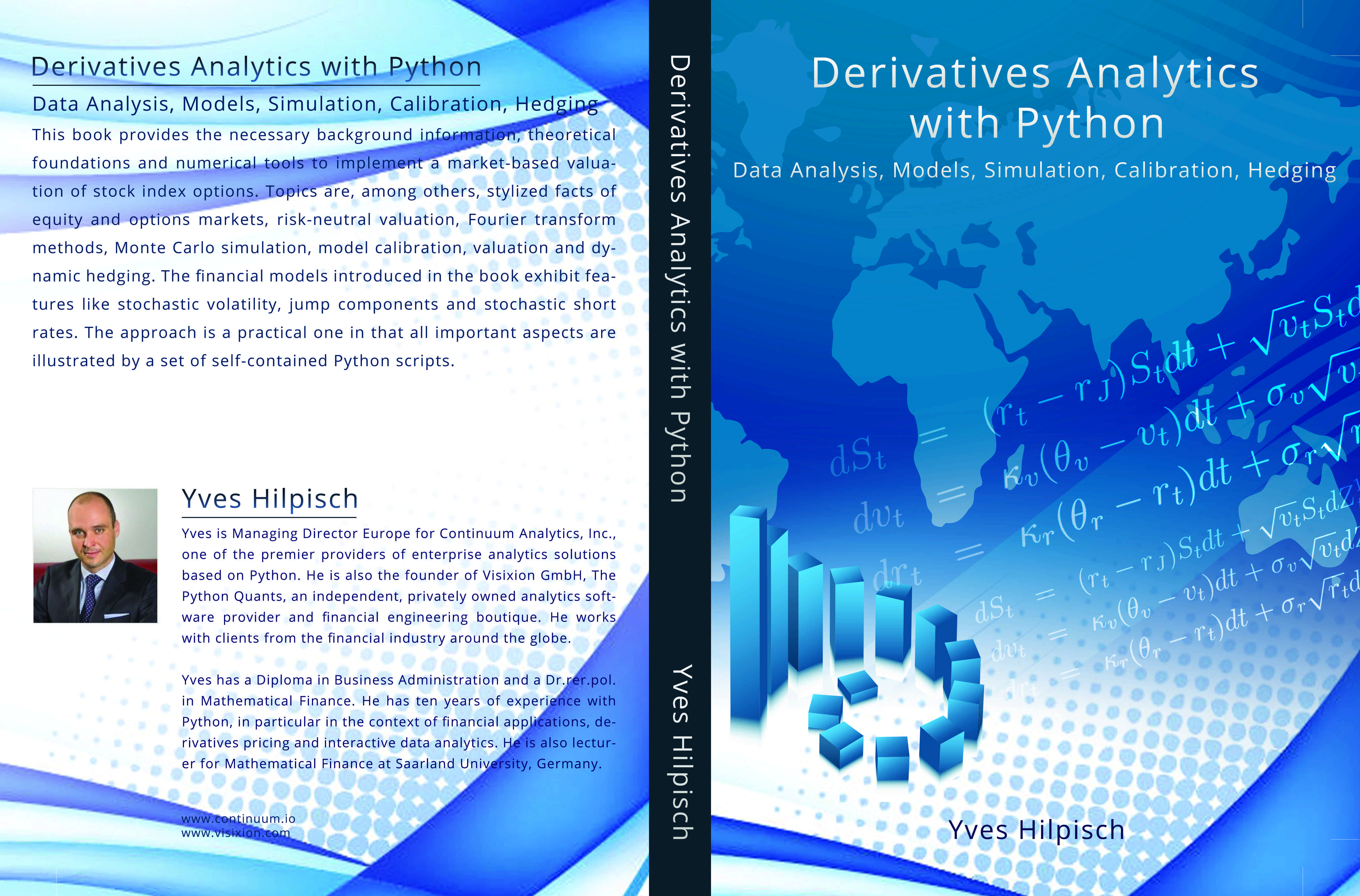
- Book (2013) "Derivatives Analytics with Python"
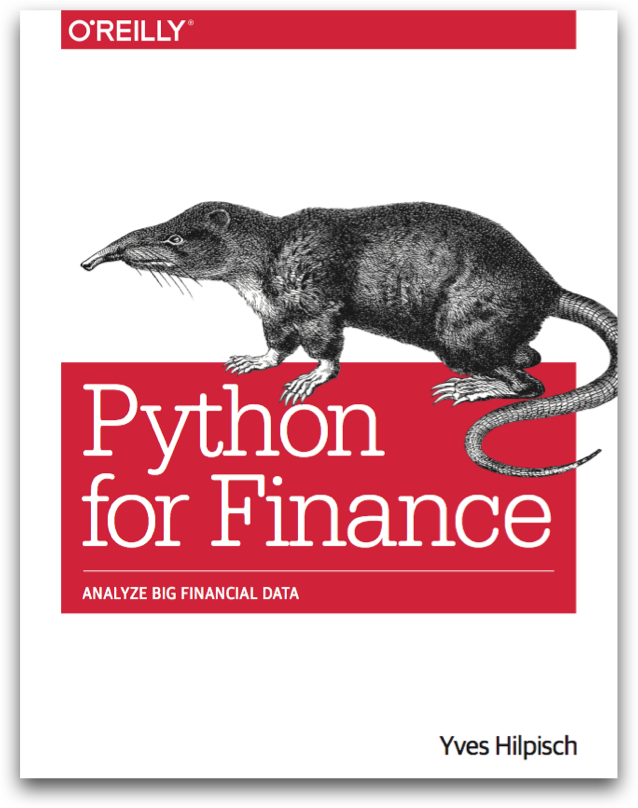
- Book (2014) "Python for Finance", O'Reilly
- Dr.rer.pol in Mathematical Finance
- Graduate in Business Administration
- Martial Arts Practitioner and Fan
See www.hilpisch.com.
Python for Derivatives Analytics
This talk focuses on
- Python for derivatives analytics
- prototyping-like algorithm implementation
- selected topics particularly relevant to finance
It does not address such important issues like
- architectural issues regarding hardware and software
- development processes, testing, documentation and production
- real world financial product modeling
- market microstructure and market conventions
- trade execution, risk management, reporting
- others like regulation
AGENDA
- Financial Algorithm Implementation
- Monte Carlo Valuation
- Binomial Option Pricing
- Performance Libraries
- Dynamic Compiling
- Parallel Code Execution
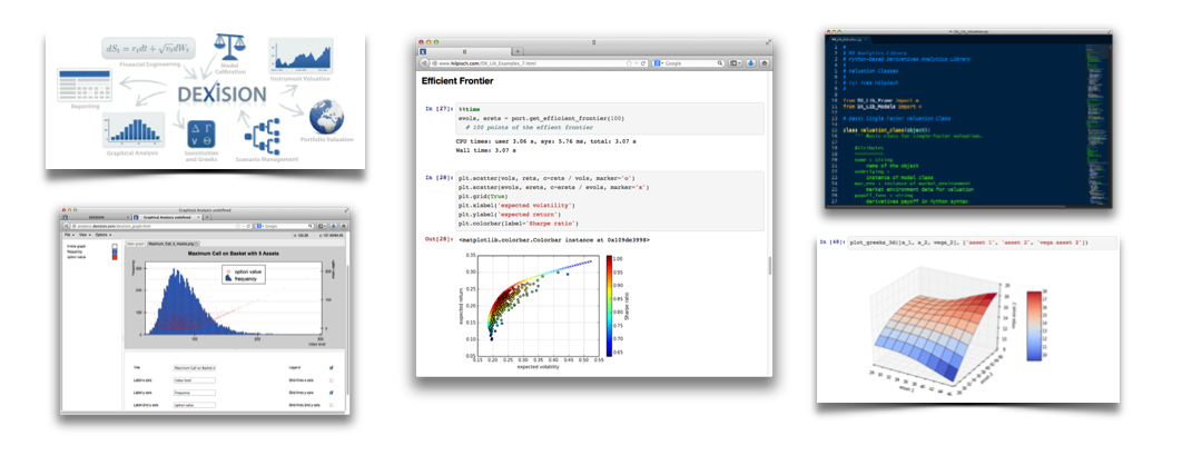
- DX Analytics
- Overview and Philosophy
- Multi-Risk Derivatives Pricing
- Global Valuation
- Web Technologies
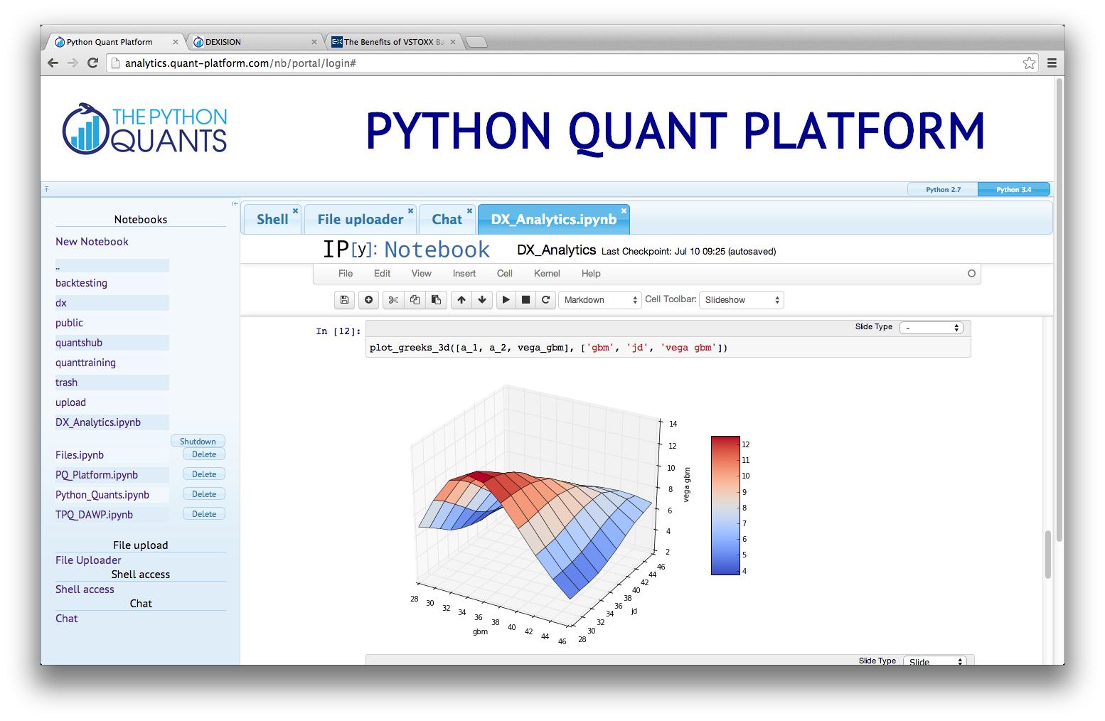
- Python Quant Platform
You can find the Slides under:
http://hilpisch.com/TPQ_Derivatives_Analytics_with_Python.html
%autosave 60
Autosaving every 60 seconds
Financial Algorithm Implementation
The majority of financial algorithms, e.g. in option pricing, can be formulated in an array (matrix) setting. It is therefore paramount to have available flexible and fast array manipulation capabilities.
NumPy provides the basic infrastructure for that. It provides the basic building blocks on which to build financial algorithms.
There are two major advantages:
- syntax: through vectorization/matrix notation, NumPy code is much more compact, easier to write, to read and to maintain
- performance: NumPy is mainly implemented in C/Fortran such that operations on the NumPy level are generally much faster than pure Python
Monte Carlo Valuation
We want to value a European call option by Monte Carlo simulation. To this end, we simulate the evolution of a stock index level which we assume to follow a geometric Brownian motion
$$dS_t = r S_t dt + \sigma S_t dZ_t$$
with $S$ the stock price, $r$ the risk-free rate, $\sigma$ the volatility and $Z$ a Brownian motion.
An exact discretization scheme is given for $t>0$ by
$$S_t = S_{t - \Delta t} \exp \left((r - \frac{1}{2} \sigma^2) \Delta t + \sigma \sqrt{\Delta t} z_t \right)$$
with $z$ being a standard normally distributed random variable.
Simulation with Pure Python
First, we import needed functions and define some global variables.
#
# Simulating Geometric Brownian Motion with Python
#
import math
from random import gauss

# Parameters
S0 = 100; r = 0.05; sigma = 0.2
T = 1.0; M = 100; dt = T / M
Then we define a function which returns us a number of I simulated index level paths.
# Simulating I paths with M time steps
def genS_py(I):
    ''' I : number of index level paths '''
    S = []
    for i in range(I):
        path = []
        for t in range(M + 1):
            if t == 0:
                path.append(S0)
            else:
                z = gauss(0.0, 1.0)
                St = path[t - 1] * math.exp((r - 0.5 * sigma ** 2) * dt
                                      + sigma * math.sqrt(dt) * z)
                path.append(St)
        S.append(path)
    return S
Let's see how long the simulation takes.
I = 100000
%time S = genS_py(I)
CPU times: user 26.7 s, sys: 240 ms, total: 27 s
Wall time: 26.6 s
A selection of the paths is easily plotted.
import matplotlib.pyplot as plt
%matplotlib inline
for i in range(5):  # first five paths
    plt.plot(S[i])
plt.xlabel('Time Steps')
plt.ylabel('Index Level')
plt.grid(True)
The Monte Carlo estimator for the European call options value with strike $K = 105$ is given by
$C_0 \approx e^{-rT} \frac{1}{I} \sum_I \max[S_T(i)-K, 0]$
In Python this might take on the form:
K = 105.
sum_val = 0.0
for path in S:
    sum_val += max(path[-1] - K, 0)
C0 = math.exp(-r * T) * sum_val / I
round(C0, 3)
8.042
However, there is a more compact way to achieve this, namely via Python's list comprehension. This is much closer to the mathematical formulation.
C0 = math.exp(-r * T) * sum([max(path[-1] - K, 0) for path in S]) / I
round(C0, 3)
8.042
Simulation with NumPy
We use the log version of the discretization scheme
$$\log S_t = \log S_{t - \Delta t} + (r - 0.5 \sigma^2 ) \Delta t + \sigma \sqrt{\Delta t} z_t $$
to fully apply NumPy's vectorization capabilities:
import numpy as np
def genS_np(I):
    ''' I : number of index level paths '''
    S = S0 * np.exp(np.cumsum((r - 0.5 * sigma ** 2) * dt
                + sigma * np.sqrt(dt)
                * np.random.standard_normal((M + 1, I)), axis=0))
    S[0] = S0
    return S
This leads to a quite compact syntax – the algorithm is fully NumPy.
It also leads to a considerable speed-up:
%time S = genS_np(I)
CPU times: user 1.1 s, sys: 140 ms, total: 1.24 s
Wall time: 1.24 s
The Monte Carlo estimator is now easily calculated as well. The NumPy syntax is really close to the mathematical formulation.
C0 = math.exp(-r * T) * np.sum(np.maximum(S[-1] - K, 0)) / I
round(C0, 3)
8.133
S = 0.0 # memory clean-up
Binomial Option Pricing with NumPy
First, the (binomial) parameters for pricing an option on a stock index level.
# Option Parameters
S0 = 100.  # initial index level
K = 105.  # strike price
T = 1.  # call option maturity
r = 0.05  # constant short rate
vola = 0.20  # constant volatility factor of diffusion

# Time Parameters
M = 1000  # time steps
dt = T / M  # length of time interval
df = math.exp(-r * dt)  # discount factor per time interval

# Binomial Parameters
u = math.exp(vola * math.sqrt(dt))  # up-movement
d = 1 / u  # down-movement
q = (math.exp(r * dt) - d) / (u - d)  # martingale probability
Binomial Option Pricing with Python Loops
The loop-heavy implementation. It is based on NumPy arrays.
import numpy as np
def oVal_py():
    # LOOP 1 - Index Levels
    S = np.zeros((M + 1, M + 1), dtype=np.float64)  # index level array
    S[0, 0] = S0
    z1 = 0
    for j in xrange(1, M + 1, 1):
        z1 += 1
        for i in xrange(z1 + 1):
            S[i, j] = S[0, 0] * (u ** j) * (d ** (i * 2))
    # LOOP 2 - Inner Values
    iv = np.zeros((M + 1, M + 1), dtype=np.float64)  # inner value array
    z2 = 0
    for j in xrange(0, M + 1, 1):
        for i in xrange(z2 + 1):
            iv[i, j] = max(S[i, j] - K, 0)
        z2 += 1
    # LOOP 3 - Valuation
    pv = np.zeros((M + 1, M + 1), dtype=np.float64)  # present value array
    pv[:, M] = iv[:, M]  # initialize last time point
    z3 = M + 1
    for j in xrange(M - 1, -1, -1):
        z3 = z3 - 1
        for i in xrange(z3):
            pv[i, j] = (q * pv[i, j + 1] + (1 - q) * pv[i + 1, j + 1]) * df
    return pv[0, 0]
The execution takes quite a bit of time.
%time C = oVal_py()
CPU times: user 3.12 s, sys: 60 ms, total: 3.18 s
Wall time: 3.01 s
round(C, 3)
8.021
Binomial Option Pricing with Numpy
The NumPy version avoids all but one loop on the Python level.
def oVal_np():
    # Index Levels with NumPy
    mu = np.arange(M + 1)
    mu = np.resize(mu, (M + 1, M + 1))
    md = np.transpose(mu)
    mu = u ** (mu - md)
    md = d ** md
    S = S0 * mu * md
    # Valuation Loop
    V = np.maximum(S - K, 0)
    Qu = np.zeros((M + 1, M + 1), dtype=np.float64)
    Qu[:, :] = q
    Qd = 1 - Qu
    z = 0
    for t in range(M - 1, -1, -1):  # backwards iteration
        V[0:M - z, t] = (Qu[0:M - z, t] * V[0:M - z, t + 1]
                        + Qd[0:M - z, t] * V[1:M - z + 1, t + 1]) * df
        z += 1
    return V[0, 0]
The NumPy version is, as expected, much faster than the Python, loop-heavy version.
%time C = oVal_np()
round(C, 3)
CPU times: user 304 ms, sys: 4 ms, total: 308 ms
Wall time: 304 ms
8.021
%timeit oVal_np()
1 loops, best of 3: 265 ms per loop
Performance Libraries
Performance Improvements through Dynamic Compiling
Numba is an open-source, NumPy-aware optimizing compiler for Python sponsored by Continuum Analytics, Inc. It uses the LLVM compiler infrastructure to compile Python byte-code to machine code especially for use in the NumPy run-time and SciPy modules.
Introductory Example
A simple example illustrates how Numba works. We start with an asymmetric nested loop:
import math
def f(n):
    result = 0.0
    for i in range(n):
        for j in range(n * i):
            result += math.sin(math.pi / 2)
    return int(result)
First, the benchmark for pure Python code.
n = 400
%time res_py = f(n)
CPU times: user 9.76 s, sys: 8 ms, total: 9.77 s
Wall time: 9.74 s
res_py # total number of loops
31920000
Second, we compile the Python function just-in-time with Numba.
import numba as nb
f_nb = nb.jit(f)
Third, we measure execution speed for the compiled version.
f_nb(n)
  # invoke one time to complete the compiling
31920000L
%timeit f_nb(n)
10 loops, best of 3: 34.4 ms per loop
The speed-up is considerable – especially given the marginal additional effort.
Binomial Option Pricing Revisited
Compiling the original function for the binomial options pricing takes only a single line of code.
oVal_nb = nb.jit(oVal_py)
The resulting speed is even higher compared to the NumPy version.
oVal_nb()
  # invoke for the first time to complete compilation
8.0210602876964057
%timeit oVal_nb()
10 loops, best of 3: 108 ms per loop
Parallel Execution with IPython
This example illustrates how to implement a parallel valuation of American options by Monte Carlo simulation. The algorithm used is the Least-Squares Monte Carlo algorithm as proposed in Longstaff-Schwartz (2001): "Valuing American Options by Simulation: A Simple Least-Squares Approach." Review of Financial Studies, Vol. 14, 113-147.
We observe speed-ups that are almost linear in the number of cores.
The LSM Algorithm
The following is an implementation of the Least-Squares Monte Carlo algorithm (LSM) of Longstaff-Schwartz (2001). You could replace it with any other function of interest ...
def optionValue(S0, vol, T, K=40, M=50, I=10 * 4096, r=0.06):
    import numpy as np
    np.random.seed(150000)  # fix the seed for every valuation
    dt = T / M  # time interval
    df = np.exp(-r * dt)  # discount factor per time time interval
    S = np.zeros((M + 1, I), dtype=np.float64)  # stock price matrix
    S[0, :] = S0  # intial values for stock price
    for t in range(1, M + 1):
        ran = np.random.standard_normal(I)
        S[t, :] = S[t - 1, :] * np.exp((r - vol ** 2 / 2) * dt
                        + vol * ran * np.sqrt(dt))
    h = np.maximum(K - S, 0)  # inner values for put option
    V = np.zeros_like(h)  # value matrix
    V[-1] = h[-1]
    for t in range(M - 1, 0, -1):
        rg = np.polyfit(S[t, :], V[t + 1, :] * df, 5)  # regression
        C = np.polyval(rg, S[t, :])  # evaluation of regression
        V[t, :] = np.where(h[t, :] > C, h[t, :],
                         V[t + 1, :] * df)  # exercise decision/optimization
    V0 = np.sum(V[1, :] * df) / I  # LSM estimator
    print "S0 %4.1f|vol %4.2f|T %2.1f| Option Value %8.3f" \
        % (S0, vol, T, V0)
    return V0
The Sequential Calculation
We want to replicate the whole table 1 of the seminal paper which contains results for 20 different parametrizations.
def seqValue():
    optionValues = []
    for S0 in (36., 38., 40., 42., 44.):  # initial stock price values
        for vol in (0.2, 0.4):  # volatility values
            for T in (1.0, 2.0):  # times-to-maturity
                optionValues.append(optionValue(S0, vol, T))
    return optionValues
Now, we measure the time for the 20 different American put options of that table 1 with sequential execution.
%time optionValues = seqValue() # calculate all values
S0 36.0|vol 0.20|T 1.0| Option Value    4.447
S0 36.0|vol 0.20|T 2.0| Option Value    4.786
S0 36.0|vol 0.40|T 1.0| Option Value    7.030
S0 36.0|vol 0.40|T 2.0| Option Value    8.384
S0 38.0|vol 0.20|T 1.0| Option Value    3.226
S0 38.0|vol 0.20|T 2.0| Option Value    3.675
S0 38.0|vol 0.40|T 1.0| Option Value    6.039
S0 38.0|vol 0.40|T 2.0| Option Value    7.553
S0 40.0|vol 0.20|T 1.0| Option Value    2.262
S0 40.0|vol 0.20|T 2.0| Option Value    2.789
S0 40.0|vol 0.40|T 1.0| Option Value    5.207
S0 40.0|vol 0.40|T 2.0| Option Value    6.794
S0 42.0|vol 0.20|T 1.0| Option Value    1.560
S0 42.0|vol 0.20|T 2.0| Option Value    2.129
S0 42.0|vol 0.40|T 1.0| Option Value    4.451
S0 42.0|vol 0.40|T 2.0| Option Value    6.126
S0 44.0|vol 0.20|T 1.0| Option Value    1.058
S0 44.0|vol 0.20|T 2.0| Option Value    1.613
S0 44.0|vol 0.40|T 1.0| Option Value    3.827
S0 44.0|vol 0.40|T 2.0| Option Value    5.507
CPU times: user 23.7 s, sys: 0 ns, total: 23.7 s
Wall time: 23.7 s
The Parallel Calculation
First, start a local cluster, if you have multiple cores in your machine.
# in the shell ...
####
# ipcluster start --n 4
####
# or maybe more cores
Second, enable IPython's parallel computing capabilities.
from IPython.parallel import Client
cluster_profile = "default"
c = Client(profile=cluster_profile)
view = c.load_balanced_view()
Again, a loop for the 20 options. This time asynchronously distributed to the multiple cores.
def parValue():
    optionValues = []
    for S in (36., 38., 40., 42., 44.):
        for vol in (0.2, 0.4):
            for T in (1.0, 2.0):
                value = view.apply_async(optionValue, S, vol, T)
                optionValues.append(value)
    c.wait(optionValues)
    return optionValues
Now, we measure the time needed with parallel execution.
%time optionValues = parValue()
CPU times: user 1.57 s, sys: 108 ms, total: 1.68 s
Wall time: 7.63 s
The speed-up is almost linear in the number of cores.
As verification, the valuation results from the parallel calculation.
for result in optionValues:
    print result.metadata['stdout'],
S0 36.0|vol 0.20|T 1.0| Option Value    4.447
S0 36.0|vol 0.20|T 2.0| Option Value    4.786
S0 36.0|vol 0.40|T 1.0| Option Value    7.030
S0 36.0|vol 0.40|T 2.0| Option Value    8.384
S0 38.0|vol 0.20|T 1.0| Option Value    3.226
S0 38.0|vol 0.20|T 2.0| Option Value    3.675
S0 38.0|vol 0.40|T 1.0| Option Value    6.039
S0 38.0|vol 0.40|T 2.0| Option Value    7.553
S0 40.0|vol 0.20|T 1.0| Option Value    2.262
S0 40.0|vol 0.20|T 2.0| Option Value    2.789
S0 40.0|vol 0.40|T 1.0| Option Value    5.207
S0 40.0|vol 0.40|T 2.0| Option Value    6.794
S0 42.0|vol 0.20|T 1.0| Option Value    1.560
S0 42.0|vol 0.20|T 2.0| Option Value    2.129
S0 42.0|vol 0.40|T 1.0| Option Value    4.451
S0 42.0|vol 0.40|T 2.0| Option Value    6.126
S0 44.0|vol 0.20|T 1.0| Option Value    1.058
S0 44.0|vol 0.20|T 2.0| Option Value    1.613
S0 44.0|vol 0.40|T 1.0| Option Value    3.827
S0 44.0|vol 0.40|T 2.0| Option Value    5.507
DX Analytics
Overview and Philosophy
DX Analytics is a Python-based derivatives analytics library, allowing for the modeling, valuation and hedging of complex multi-risk, multi-derivatives portfolios/trades. General ideas and approaches:
- general risk-neutral valuation ("Global Valuation")
- Monte Carlo simulation for valuation, Greeks
- Fourier-based formulae for calibration
- arbitrary models for stochastic processes
- single & multi risk derivatives
- European and American exercise
- completely implemented in Python
- hardware not a limiting factor
Global Valuation at its core:
- non-redundant modeling (e.g. of risk factors)
- consistent simulation (e.g. given correlations)
- consistent value and risk aggregation (e.g. full re-valuation)
- single positions or consistent portfolio view
Multi-Risk Derivative Case Study
First, we need to import the classes and functions of the library.
from dx import *
%matplotlib inline
Risk-Neutral Discounting
The discounting class is central for risk-neutral pricing.
# constant short rate
r = constant_short_rate('r', 0.02)
time_list = pd.date_range(start='2014/6/1',
                end='2014/12/31', freq='M').to_pydatetime()
r.get_discount_factors(time_list) # unit zero-coupon bond values
array([[datetime.datetime(2014, 6, 30, 0, 0), 0.98996846313427345],
       [datetime.datetime(2014, 7, 31, 0, 0), 0.99165148240937606],
       [datetime.datetime(2014, 8, 31, 0, 0), 0.99328293498780673],
       [datetime.datetime(2014, 9, 30, 0, 0), 0.99497158910909278],
       [datetime.datetime(2014, 10, 31, 0, 0), 0.99660850388541455],
       [datetime.datetime(2014, 11, 30, 0, 0), 0.99830281171867608],
       [datetime.datetime(2014, 12, 31, 0, 0), 1.0]], dtype=object)
Market Environment
Our market consists of two risk factors.
# market environments
me_gbm = market_environment('gbm', dt.datetime(2014, 1, 1))
me_jd = market_environment('jd', dt.datetime(2014, 1, 1))
Market environment for geometric Brownian motion.
# geometric Brownian motion
me_gbm.add_constant('initial_value', 36.)
me_gbm.add_constant('volatility', 0.2)
me_gbm.add_constant('currency', 'EUR')
me_gbm.add_constant('model', 'gbm')
Market environment for jump diffusion.
# jump diffusion
me_jd.add_constant('initial_value', 36.)
me_jd.add_constant('volatility', 0.2)
me_jd.add_constant('lambda', 0.5)
    # probability for jump p.a.
me_jd.add_constant('mu', -0.75)
    # expected jump size [%]
me_jd.add_constant('delta', 0.1)
    # volatility of jump
me_jd.add_constant('currency', 'EUR')
me_jd.add_constant('model', 'jd')
You can share common constants and curves by adding whole market environment objects to another one.
# valuation environment
val_env = market_environment('val_env', dt.datetime(2014, 1, 1))
val_env.add_constant('paths', 5000)
val_env.add_constant('frequency', 'W')
val_env.add_curve('discount_curve', r)
val_env.add_constant('starting_date', dt.datetime(2014, 1, 1))
val_env.add_constant('final_date', dt.datetime(2014, 12, 31))
# add valuation environment to market environments
me_gbm.add_environment(val_env)
me_jd.add_environment(val_env)
We have now our market together. What is still missing are correlations.
underlyings = {
               'gbm' : me_gbm,
               'jd' : me_jd
               }
correlations = [
                ['gbm', 'jd', 0.75],
                ]
Risk Factors
We need to instantiate two model classes to get our risk factors, given the market environments.
gbm = geometric_brownian_motion('gbm_obj', me_gbm)
jd = jump_diffusion('jd_obj', me_jd)
European Max Call Option
The environment for the derivative.
me_max_call = market_environment('put', dt.datetime(2014, 1, 1))
me_max_call.add_constant('maturity', dt.datetime(2014, 12, 31))
me_max_call.add_constant('currency', 'EUR')
me_max_call.add_environment(val_env)
The payoff definition is a Python string that can be evaluated by Python.
payoff_call = "np.maximum(np.maximum(maturity_value['gbm'], "
payoff_call += "maturity_value['jd']) - 34., 0)"
Valuation by Simulation
To value the derivative, we need to instantiate an appropriate valuation class.
max_call = valuation_mcs_european_multi(
                        name='max_call',
                        val_env=me_max_call,
                        assets=underlyings,
                        correlations=correlations,
                        payoff_func=payoff_call)
Value and Greeks are now only one method call away.
max_call.present_value()
5.132973
max_call.delta('gbm')
0.5421319444444449
max_call.vega('jd')
5.634100000000064
Graphical Analysis
Let us generate a somehow broader overview of the option statistics. We start with the present value of the option given different initial values for the two underlyings.
asset_1 = np.arange(28., 46.1, 2.)
asset_2 = asset_1
a_1, a_2 = np.meshgrid(asset_1, asset_2)
value = np.zeros_like(a_1)
len(value.flatten()) # number of values
100
%%time
for i in range(np.shape(value)[0]):
    for j in range(np.shape(value)[1]):
        max_call.update('gbm', initial_value=a_1[i, j])
        max_call.update('jd', initial_value=a_2[i, j])
        value[i, j] = max_call.present_value()
CPU times: user 5.87 s, sys: 0 ns, total: 5.87 s
Wall time: 5.87 s
And the graphical representation of the option present values.
plot_greeks_3d([a_1, a_2, value], ['gbm', 'jd', 'present value'])
Now the surfaces for the Greeks. Delta values first (jd).
delta_jd = np.zeros_like(a_1)
%%time
for i in range(np.shape(delta_jd)[0]):
    for j in range(np.shape(delta_jd)[1]):
        max_call.update('gbm', initial_value=a_1[i, j])
        max_call.update('jd', initial_value=a_2[i, j])
        delta_jd[i, j] = max_call.delta('jd')
CPU times: user 15.2 s, sys: 372 ms, total: 15.5 s
Wall time: 15.6 s
The surface for the jd Delta.
plot_greeks_3d([a_1, a_2, delta_jd], ['gbm', 'jd', 'delta jd'])
Next, the surface for the Vega (gbm).
vega_gbm = np.zeros_like(a_1)
%%time
for i in range(np.shape(vega_gbm)[0]):
    for j in range(np.shape(vega_gbm)[1]):
        max_call.update('gbm', initial_value=a_1[i, j])
        max_call.update('jd', initial_value=a_2[i, j])
        vega_gbm[i, j] = max_call.vega('gbm')
CPU times: user 7.45 s, sys: 80 ms, total: 7.53 s
Wall time: 7.54 s
The surface for the gbm Vega.
plot_greeks_3d([a_1, a_2, vega_gbm], ['gbm', 'jd', 'vega gbm'])
Global Valuation
Let us check what impact a change in the correlation has. First the benchmark present value.
# reset initial values
max_call.update('gbm', initial_value=36.)
max_call.update('jd', initial_value=36.)
max_call.present_value()
5.132973
We are in a positive correlation case.
path_no = 1
paths1 = max_call.underlying_objects['gbm'].get_instrument_values()[:, path_no]
paths2 = max_call.underlying_objects['jd'].get_instrument_values()[:, path_no]

plt.figure(figsize=(9, 5))
plt.plot(max_call.time_grid, paths1, 'r', label='gbm')
plt.plot(max_call.time_grid, paths2, 'b', label='jd')
plt.gcf().autofmt_xdate()
plt.legend(loc=0); plt.grid(True)
# positive correlation case
Now change to a negative correlation case.
correlations = [
                ['gbm', 'jd', -0.75],
                ]
max_call = valuation_mcs_european_multi(
                        name='max_call',
                        val_env=me_max_call,
                        assets=underlyings,
                        correlations=correlations,
                        payoff_func=payoff_call)
The value increases (as expected) ...
max_call.present_value()
6.599296
... and our singled-out paths show the correlation effect graphically.
paths1 = max_call.underlying_objects['gbm'].get_instrument_values()[:, path_no]
paths2 = max_call.underlying_objects['jd'].get_instrument_values()[:, path_no]

plt.figure(figsize=(9, 5))
plt.plot(max_call.time_grid, paths1, 'r', label='gbm')
plt.plot(max_call.time_grid, paths2, 'b', label='jd')
plt.gcf().autofmt_xdate()
plt.legend(loc=0); plt.grid(True)
# negative correlation case
Parallel Valuation of Large Derivatives Portfolio
from dx import *
Market environment and simulation object for underlying risk factor (stock).
r = constant_short_rate('r', 0.06)

me_gbm = market_environment('gbm', dt.datetime(2015, 1, 1))
me_gbm.add_constant('initial_value', 36.)
me_gbm.add_constant('volatility', 0.2)
me_gbm.add_constant('currency', 'EUR')
me_gbm.add_constant('model', 'gbm')

underlyings = {'gbm' : me_gbm}
Market environment for American put option as well as 100 options positions.
me_put = market_environment('put', dt.datetime(2015, 1, 1))
me_put.add_constant('maturity', dt.datetime(2015, 12, 31))
me_put.add_constant('strike', 40.)
me_put.add_constant('currency', 'EUR')
Valuation environment and 100 options positions.
val_env = market_environment('val_env', dt.datetime(2015, 1, 1))
val_env.add_constant('paths', 25000)
val_env.add_constant('frequency', 'M')
val_env.add_curve('discount_curve', r)
val_env.add_constant('starting_date', dt.datetime(2015, 1, 1))
val_env.add_constant('final_date', dt.datetime(2015, 12, 31))
positions = {}
for i in range(100):
    positions[i] = derivatives_position('am_put_pos', 2, ['gbm'], me_put,
                   'American single', 'np.maximum(40 - instrument_values, 0)')
The sequential valuation.
port_sequ = derivatives_portfolio('portfolio', positions, val_env,
                        underlyings, correlations=None, parallel=False)
%time res = port_sequ.get_values()
CPU times: user 8.91 s, sys: 408 ms, total: 9.32 s
Wall time: 9.33 s
res[:2]
| position | name | quantity | value | currency | pos_value | |
|---|---|---|---|---|---|---|
| 0 | 0 | am_put_pos | 2 | 4.409607 | EUR | 8.819214 |
| 1 | 1 | am_put_pos | 2 | 4.424785 | EUR | 8.849570 |
The parallel valuation.
port_para = derivatives_portfolio('portfolio', positions, val_env,
                        underlyings, correlations=None, parallel=True)
%time res = port_para.get_values()
  # parallel valuation with 4 cores
CPU times: user 100 ms, sys: 548 ms, total: 648 ms
Wall time: 3 s
res[:2]
| position | name | quantity | value | currency | pos_value | |
|---|---|---|---|---|---|---|
| 0 | 0 | am_put_pos | 2 | 4.405225 | EUR | 8.81045 |
| 1 | 1 | am_put_pos | 2 | 4.405225 | EUR | 8.81045 |
Web Technologies for Derivatives Analytics
Financial application building faces some challanges:
- time-to-market: financial market realities demand for ever faster times-to-market when it comes to new applications and functionality
- maintainability: applications must be maintainable over longer periods of time at reasonable costs
- deployment: deployment on a global scale and sometimes on thousands of machines is often required
- scalability: computational workloads are continuously increasing – demanding for flexible scalability
Web technologies provide to some extent better solutions to these problems than traditional architectures.
In what follows we want to implement a Web service-based valuation engine for volatility options. The valuation model is the one Gruenbichler-Longstaff (1996). They model the volatility process (e.g. the process of a volatility index) in direct fashion by a square-root diffusion:
$$dV_t = \kappa_V (\theta_V - V_t)dt + \sigma_V \sqrt{V_t} dZ$$
The variables and parameters have the following meanings:
- $V_t$ is the time $t$ value of the volatility index, for example the VSTOXX
- $\theta_V$ is the long-run mean of the volatility index
- $\kappa_V$ is the rate at which $V_t$ reverts to $\theta$
- $\sigma_V$ is the volatility of the volatility ("vol-vol")
- $\theta_V, \kappa_V, \sigma_V$ are assumed to be constant and positive
- $Z_t$ is a standard Brownian motion
In this model, Gruenbichler and Longstaff (1996) derive the following formula for the value of a European call option on volatility. In the formula, $D(T)$ is the appropriate discount factor. The parameter $\zeta$ denotes the expected premium for volatility risk while $Q(\cdot)$ is the complementary non-central $\chi^2$ distribution.
$$ \begin{eqnarray*} C(V_0,K,T) &=& D(T)\cdot e^{- \beta T} \cdot V_0 \cdot Q(\gamma \cdot K | \nu + 4, \lambda)\\ &+& D(T)\cdot \left(\frac{\alpha}{\beta}\right) \cdot \left(1-e^{- \beta T}\right) \cdot Q(\gamma \cdot K | \nu+2, \lambda) \\ &-& D(T) \cdot K \cdot Q(\gamma \cdot K | \nu, \lambda) \\ \alpha &=& \kappa \theta \\ \beta &=& \kappa + \zeta \\ \gamma &=& \frac{4 \beta}{\sigma^2 \left(1-e^{- \beta T}\right)} \\ \nu &=& \frac{4 \alpha}{\sigma^2} \\ \lambda &=& \gamma \cdot e^{- \beta T} \cdot V \end{eqnarray*} $$
In Python, the valuation formula might take on the form of the function calculate_option_value.
#
# Valuation of European volatility call options
# vol_pricing_formula.py
#
from scipy.stats import ncx2
import numpy as np

def calculate_option_value(V0, kappa, theta, sigma, zeta, T, r, K):
    D = np.exp(-r * T)  # discount factor
    # variables
    alpha = kappa * theta
    beta = kappa + zeta
    gamma = 4 * beta / (sigma ** 2 * (1 - np.exp(-beta * T)))
    nu = 4 * alpha / sigma ** 2
    lamb = gamma * np.exp(-beta * T) * V0
    cx1 = 1 - ncx2.cdf(gamma * K, nu + 4, lamb)
    cx2 = 1 - ncx2.cdf(gamma * K, nu + 2, lamb)
    cx3 = 1 - ncx2.cdf(gamma * K, nu, lamb)
    # formula for European call price
    value = (D * np.exp(-beta * T) * V0 * cx1
      + D * (alpha / beta) * (1 - np.exp(-beta * T))
      * cx2 - D * K * cx3)
    return value
To simplify the implementation of the Web service, consider this second Python script with the convenience function get_option_value.
#
# Valuation of European volatility options
# vol_pricing_service.py
#
from volservice import calculate_option_value
# model parameters
PARAMS={'V0' : 'current volatility level', 'kappa' : 'mean-reversion factor',
    'theta' : 'long-run mean of volatility', 'sigma' : 'volatility of volatility',
    'zeta' : 'factor of the expected volatility risk premium',
    'T' : 'time horizon in years', 'r' : 'risk-free interest rate',
    'K' : 'strike'}
def get_option_value(data):
    errorline = 'Missing parameter %s (%s)\n'
    errormsg = ''
    for para in PARAMS:
        if not data.has_key(para):
            # check if all parameters are provided
            errormsg += errorline % (para, PARAMS[para])
    if errormsg != '':
        return errormsg
    else:
        result = calculate_option_value(
                float(data['V0']), float(data['kappa']), float(data['theta']),
                float(data['sigma']), float(data['zeta']), float(data['T']),
                float(data['r']), float(data['K']))
        return str(result)
The core function are there, we need to wrap it in a Web application. To simplify this task, we use Werkzeug, a tool for better handling of WSGI applications.
#
# Valuation of European volatility options
# vol_pricing.py
#
from volservice import get_option_value
from werkzeug.wrappers import Request, Response
from werkzeug.serving import run_simple

def application(environ, start_response):
    request = Request(environ)
      # wrap environ in new object
    text = get_option_value(request.args)
      # provide all paramters of the call to function
      # get back either error message or option value
    response = Response(text, mimetype='text/html')
      # generate response object based on the returned text
    return response(environ, start_response)

# if __name__=='__main__':
#    run_simple('localhost', 4000, application)
Execute the script vol_pricing.py in a separate (I)Python kernel. And you are ready to go.
$ python volservice/vol_pricing.py
* Running on http://localhost:4000/
You can now either use the browser for the Web service or you can do it interactively (by scripting).
import numpy as np
from urllib import urlopen
url = 'http://localhost:4000/'
Simply calling the Web service without providing any parameter value generates a number of error messages.
print urlopen(url).read()
Missing parameter V0 (current volatility level)
Missing parameter r (risk-free interest rate)
Missing parameter kappa (mean-reversion factor)
Missing parameter T (time horizon in years)
Missing parameter theta (long-run mean of volatility)
Missing parameter zeta (factor of the expected volatility risk premium)
Missing parameter sigma (volatility of volatility)
Missing parameter K (strike)
Let us use a URL string to parameterize the Web service call.
urlpara = 'http://localhost:4000/application?V0=25&kappa=2.0'
urlpara += '&theta=25&sigma=1.0&zeta=0.0&T=1&r=0.02&K={}'
  # K is to be parameterized
This makes the valuation of a volatility call option for 250 different strikes quite convenient.
%%time
strikes = np.linspace(20, 30, 250)
results = []
for K in strikes:
    option_value = float(urlopen(urlpara.format(K)).read())
      # get option value from Web service given K
    results.append(option_value)
results = np.array(results)
CPU times: user 184 ms, sys: 40 ms, total: 224 ms
Wall time: 537 ms
The graphical representation of the valuation results.
import matplotlib.pyplot as plt
%matplotlib inline
plt.plot(strikes, results, 'r.')
plt.grid(True)
plt.xlabel('strike')
plt.ylabel('European call option value')
<matplotlib.text.Text at 0x7fecab8ef850>
Python Quant Platform
Why Python for Derivatives Analytics?
10 years ago, Python was considered exotic in Finance – at best. Today, Python has become a major force in Finance due to a number of characteristics:
- syntax: Python syntax is pretty close to the symbolic language used in mathematical finance (also: symbolic Python with SymPy)
- multi-purpose: prototyping, development, production, sytems administration – Python is one for all
- libraries: there is a library for almost any task or problem you face
- efficiency: Python speeds up all IT development tasks financial institutions typically face and reduces maintenance costs
- performance: Python has evolved from a scripting language to a 'meta' language with bridges to all high performance environments (e.g. LLVM, multi-core CPUs, GPUs, clusters)
- interoperability: Python seamlessly integrates with almost any other language and technology
- interactivity: Python allows domain experts to get closer to their business and financial data pools and to do interactive real-time analytics
- collaboration: tools like Python Quant Platform (http://quant-platform.com) allow developers and financial data scientists to collaborate across companies and business departments, to share code, data and their analytics insights easily

www.hilpisch.com | www.pythonquants.com
Python for Finance – my NEW book (out as Early Release)
Derivatives Analytics with Python – my derivatives analytics book
