Python and the Financial Community
A Subjective and Biased Overview
The Python Language
Black-Scholes-Merton (1973) SDE of geometric Brownian motion.
$$ dS_t = rS_tdt + \sigma S_t dZ_t $$
Monte Carlo simulation: draw $I$ standard normally distributed random number $z_t^i$ and apply them to the following by Euler disctretization scheme to simulate $I$ end values of the GBM:
$$ S_{T} = S_0 \exp \left(\left( r - \frac{1}{2} \sigma^2\right) T + \sigma \sqrt{T} z_T \right) $$
Latex description of Euler discretization.
S_T = S_0 \exp (( r - 0.5 \sigma^2 ) T + \sigma \sqrt{T} z_T)
Python implementation of algorithm.
from pylab import *
S0 = 100.; r = 0.01; T = 0.5; sigma = 0.2
ST = S0 * exp((r - 0.5 * sigma ** 2) * T
     + sigma * sqrt(T) * standard_normal(10000))
Interactive visualization of simulation results.
%matplotlib inline
hist(ST, bins=40);
grid(True)
The Python Ecosystem
- IPython (Notebook)
- NumPy (fast, vectorized array operations)
- SciPy (collection of scientific classes/functions)
- pandas (times series and tabular data)
- PyTables (hardware-bound IO operations)
- scikit-learn (machine learning algorithms)
- statsmodels (statistical classes/functions)
- xlwings (Python-Excel integration)
Financial Libraries
By others:
- zipline (backtesting of trading algos)
- matplotlib.finance (financial plots)
- Python wrappers (QuantLib)
By us:
- DEXISION – GUI-based financial engineering
- DX Analytics – global valuation of multi-risk derivatives and portfolios
APIs
- OANDA (fx trading platform)
- Thomson Reuters (wrapper for unified API in the making)
- ...
Integration
- C/C++ (natively)
- Julia (IPython)
- JavaScript (IPython)
- R (IPython/rpy2)
- Matlab (NumPy)
- ...
Pushing data from Python to R.
%load_ext rpy2.ipython
X = arange(100)
Y = 2 * X + 5 + 2 * standard_normal(len(X))
%Rpush X Y
Generating plots with R.
%R plot(X, Y, pch=19, col='blue'); grid(); title("R Plot with IPython")
Doing statistics in R.
%R print(summary(lm(Y~X)))
Call:
lm(formula = Y ~ X)

Residuals:
    Min      1Q  Median      3Q     Max
-4.6160 -1.3221  0.0707  1.2701  5.5099

Coefficients:
            Estimate Std. Error t value Pr(>|t|)
(Intercept) 4.973043   0.415827   11.96   <2e-16 ***
X           2.000921   0.007257  275.73   <2e-16 ***
---
Signif. codes:  0 ‘***’ 0.001 ‘**’ 0.01 ‘*’ 0.05 ‘.’ 0.1 ‘ ’ 1

Residual standard error: 2.095 on 98 degrees of freedom
Multiple R-squared:  0.9987,	Adjusted R-squared:  0.9987
F-statistic: 7.603e+04 on 1 and 98 DF,  p-value: < 2.2e-16
Pulling data from R to Python.
%R c = coef(lm(Y~X))
%Rpull c
c
<FloatVector - Python:0x10b211b90 / R:0x1017576a8>
[4.973043, 2.000921]
Performance
Finance algorithms are loop-heavy; Python loops are slow; Python is too slow for finance.
def counting_py(N):
    s = 0
    for i in xrange(N):
        for j in xrange(N):
            s += int(cos(log(1)))
    return s
N = 2000
%time counting_py(N)
# memory efficient but slow
CPU times: user 19 s, sys: 18.7 ms, total: 19.1 s
Wall time: 19.1 s
4000000
First approach: vectorization with NumPy.
%%time
arr = ones((N, N))
print int(sum(cos(log(arr))))
# much faster but NOT memory efficient
4000000
CPU times: user 96.6 ms, sys: 54.9 ms, total: 151 ms
Wall time: 153 ms
arr.nbytes
32000000
Second approach: dynamic compiling with Numba.
import numba
counting_nb = numba.jit(counting_py)
%time counting_nb(N)
CPU times: user 152 ms, sys: 23.6 ms, total: 176 ms
Wall time: 220 ms
4000000
%timeit counting_nb(N)
# even faster AND memory efficient
10 loops, best of 3: 54.5 ms per loop
Hardware-bound IO operations are standard for Python.
arr = standard_normal((12500, 10000))
arr.nbytes
# a giga byte worth of data
1000000000
%time save('data', arr)
CPU times: user 55.1 ms, sys: 1.85 s, total: 1.91 s
Wall time: 2.35 s
!ls -n data*
-rw-r--r-- 1 501 20 1000000080 22 Sep 16:14 data.npy
!rm data*
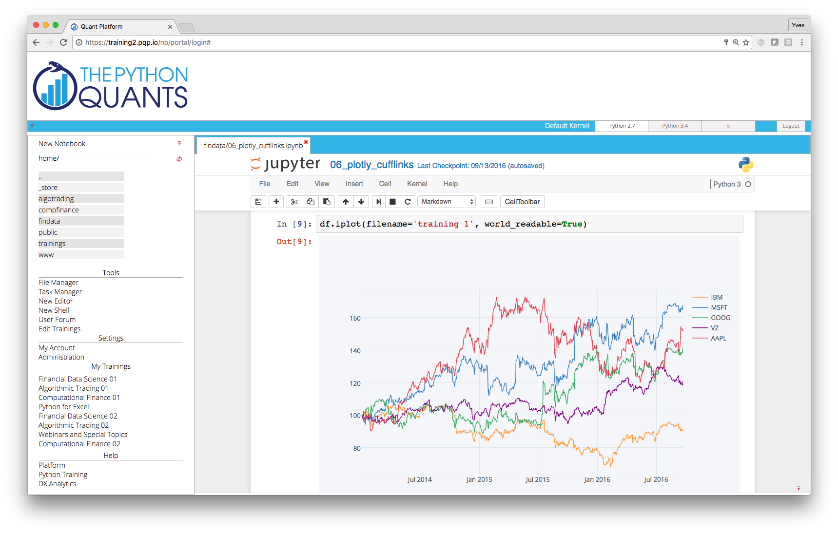
Python Quant Platform
Integrating it all and adding collaboration and scalability (http://quant-platform.com).

The Large Banks
- Bank of America Merill Lynch (Quartz platform)
- JPMorgan Chase (Athena platform)
- ...
The Hedge Funds
- AQR Capital Management (origin of pandas)
- Two Sigma Investments (large scale data analytics)
- ARC Investments (full-fledged Python for vol trading)
- ...
Innovators in the Space
- Quantopian (algo trading & backtesting)
- Washington Square Technologies (trade & risk platform)
- Deutsche Boerse/Eurex (VSTOXX and Variance Advanced Services)
- ...
Python-based tutorials by Eurex (http://www.eurexchange.com/vstoxx/).

Books
By others:
- Python for Financial Modelling @ Wiley Finance (2009)
- Python for Finance @ Packt Publishing (2014)
By myself:
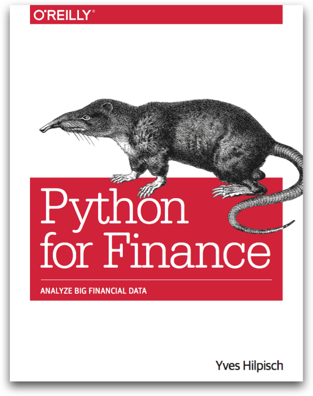
- Python for Finance – Analyze Big Financial Data @ O'Reilly (2014)
- Derivatives Analytics with Python @ Wiley Finance (2015)
Integrated offering: book + notebooks + platform + training + ...

Financial Research
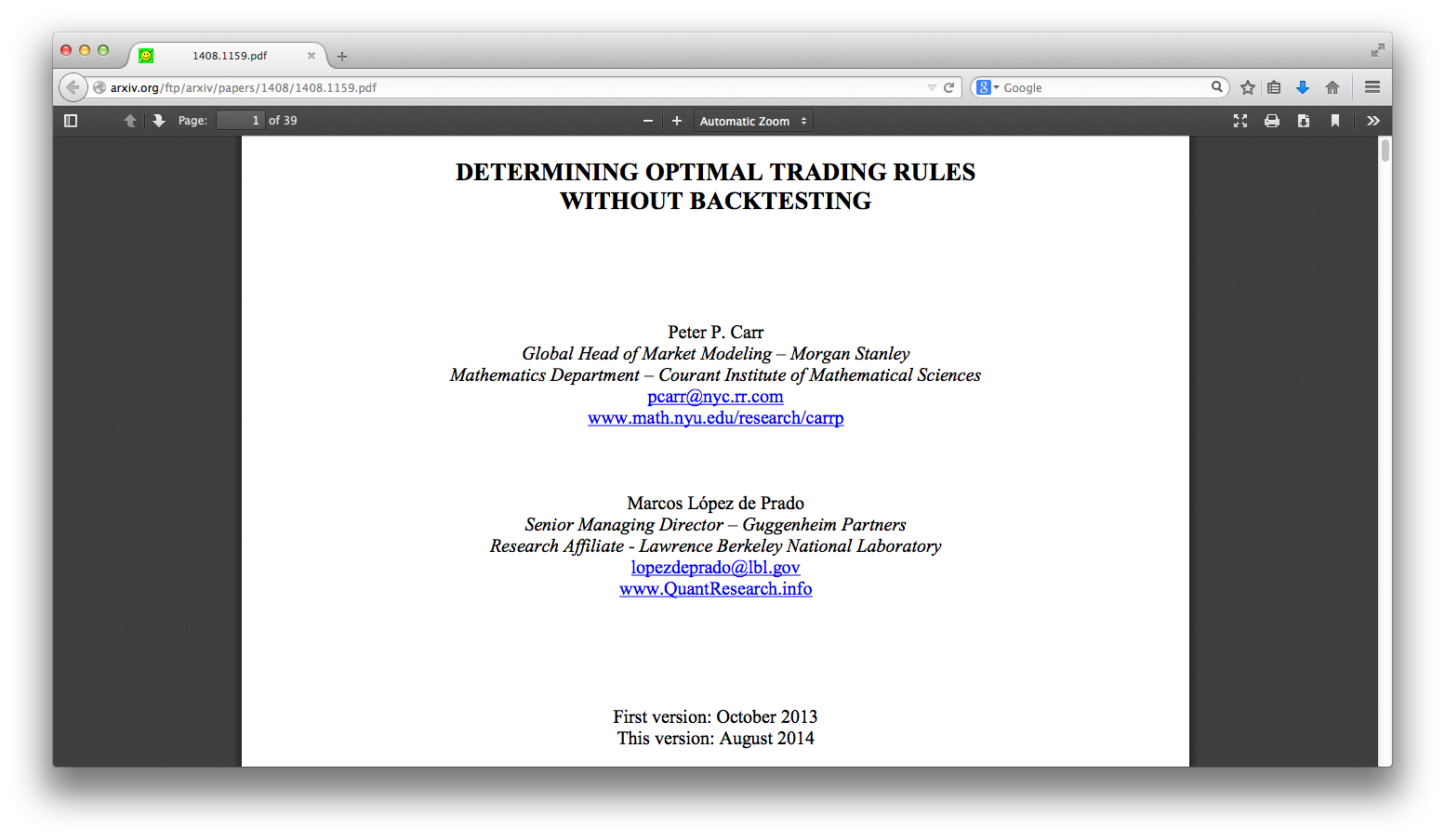
"The appendices present an implementation in Python of our experiments." (p. 3)

Education
- Master of Financial Engineering @ Baruch College CUNY
- Master of Data Science @ City University of New York
- Numerical Option Pricing with Python @ Saarland University
- ...
"Knowledge and Skills: Our graduates have working experience with C++, VBA, Python, R, and Matlab for financial applications. They share an exceptionally strong work ethic and possess excellent interpersonal, teamwork, and communication skills."
Training
By others:
- Python for Finance @ Continuum Analytics
- Python for Finance @ Enthought
By myself:
- Python for Quant Finance @ Python for Quant Finance Meetup Group
- Python for Finance @ http://quantshub.com
- NumPy & pandas for Finance @ CQF Institute/Fitch Learnings
- ...
Meetups
For Python Quants Conference
- 1st conference in New York City on 14. March 2014
- 2nd conference in London on 28. November 2014
- 3rd conference planned for QI 2015 in Asia (eg Shanghai)
Contact us
Please contact us if you have any questions or want to get involved in our Python community events.

Python Quant Platform | http://quant-platform.com
Derivatives Analytics with Python | Derivatives Analytics @ Wiley Finance
Python for Finance | Python for Finance @ O'Reilly