Browser-based, Collaborative Financial & Derivatives Analytics
Python Quant Platform and DX Analytics
Dr. Yves J. Hilpisch | The Python Quants GmbH
analytics@pythonquants.com | www.pythonquants.com
For Python Quants Conference, 28. November 2014
The Python Language
Black-Scholes-Merton (1973) SDE of geometric Brownian motion. The "Hello World example of Quant Finance."
$$ dS_t = rS_tdt + \sigma S_t dZ_t $$
Monte Carlo simulation: draw $I$ standard normally distributed random number $z_t^i$ and apply them to the following by Euler disctretization scheme to simulate $I$ end values of the GBM:
$$ S_{T} = S_0 \exp \left(\left( r - \frac{1}{2} \sigma^2\right) T + \sigma \sqrt{T} z_T \right) $$
Latex description of Euler discretization.
S_T = S_0 \exp (( r - 0.5 \sigma^2 ) T + \sigma \sqrt{T} z_T)
Python implementation of algorithm.
from pylab import *
S_0 = 100.; r = 0.01; T = 0.5; sigma = 0.2
z_T = standard_normal(10000)
S_T = S_0 * exp((r - 0.5 * sigma ** 2) * T + sigma * sqrt(T) * z_T)
Again, Latex for comparison:
S_T = S_0 \exp (( r - 0.5 \sigma^2 ) T + \sigma \sqrt{T} z_T)
Interactive visualization of simulation results.
%matplotlib inline
pyfig = figure()
hist(S_T, bins=40);
grid()

The Python Ecosystem
The Python ecosystem can be considered one of the major competitive advantages of the language.
- IPython (Notebook)
- NumPy (fast, vectorized array operations)
- SciPy (collection of scientific classes/functions)
- pandas (times series and tabular data)
- PyTables (hardware-bound IO operations)
- scikit-learn (machine learning algorithms)
- statsmodels (statistical classes/functions)
- xlwings (Python-Excel integration)
Integration – No "Either Or" with Python
Python integrates pretty well with almost any other language used for scientific and financial computing.
- C/C++ (natively)
- Julia (IPython)
- JavaScript (IPython)
- R (IPython/rpy2)
- Matlab (NumPy)
- ...
Example: Statistics with R
We analyze the statistical correlation between the EURO STOXX 50 stock index and the VSTOXX volatility index.
First, reading the EURO STOXX 50 & VSTOXX data.
import pandas as pd
es = pd.HDFStore('data/SX5E.h5', 'r')['SX5E']
vs = pd.HDFStore('data/V2TX.h5', 'r')['V2TX']
es['SX5E'].plot(figsize=(9, 6))

Generating log returns with Python and pandas.
import numpy as np
# log returns for the major indices' time series data
datv = pd.DataFrame({'SX5E' : es['SX5E'], 'V2TX': vs['V2TX']}).dropna()
rets = np.log(datv / datv.shift(1)).dropna()
ES = rets['SX5E'].values
VS = rets['V2TX'].values
Bridging to R from within IPython Notebook and pushing Python data to the R run-time.
%load_ext rpy2.ipython
%Rpush ES VS
Plotting with R in IPython Notebook.
%R plot(ES, VS, pch=19, col='blue'); grid(); title("Log returns ES50 & VSTOXX")

Linear regression with R.
%R c = coef(lm(VS~ES))
%R print(summary(lm(VS~ES)))
Regression line visualized.
%R plot(ES, VS, pch=19, col='blue'); grid(); abline(c, col='red', lwd=5)

Pulling data from R to Python and using it.
%Rpull c
plt.figure(figsize=(9, 6))
plt.plot(ES, VS, 'b.')
plt.plot(ES, c[0] + c[1] * ES, 'r', lw=3)
plt.grid(); plt.xlabel('ES'); plt.ylabel('VS')

If you want to have it nicer, interactive and embeddable anywhere – use plot.ly
import plotly.plotly as ply
ply.sign_in('yves', 'token')
Let us generate a plot with fewer data points.
pyfig = plt.figure(figsize=(9, 6)); n = 100
plt.plot(ES[:n], VS[:n], 'b.')
plt.plot(ES[:n], c[0] + c[1] * ES[:n], 'r', lw=3)
plt.grid(); plt.xlabel('ES'); plt.ylabel('VS')

Only single line of code needed to convert matplotlib plot into interactive D3 plot.
ply.iplot_mpl(pyfig) # convert mpl plot into interactive D3
Example: Working with Julia
Julia is, for example, often faster for recursive function formulations. As an example, consider the Fibonacci sequence.
# quite slow in Python
def fib_rec(n):
    if n < 2:
        return n
    else:
        return fib_rec(n - 1) + fib_rec(n - 2)
%time fib_rec(35)
%%julia
# much faster in Julia
fib_rec(n) = n < 2 ? n : fib_rec(n - 1) + fib_rec(n - 2)
@elapsed fib_rec(35)
For comparison, an iterative function implementation.
# iterative version in Python
def fib_it(n):
    x,y = 0, 1
    for i in xrange(1, n + 1):
        x, y = y, x + y
    return x
%time fn = fib_it(1000000)  # with 1,000,000
%%julia
# iterative version in Julia
function fib_it(n)
  x, y = (0,1)
  for i = 1:n
    x, y = (y, x + y)
  end
  return x
end
fib_it(5)  # initial call
@elapsed fib_it(10000000)  # with 10,000,000
For final comparison, the dynamically compiled Python version with Numba.
import numba
fib_nb = numba.jit(fib_it)
%timeit fib_nb(10000000)  # with 10,000,000
Performance – Numerical Algorithms
Finance algorithms are loop-heavy; Python loops are slow; Python is too slow for finance.
def counting_py(N):
    s = 0
    for i in xrange(N):
        for j in xrange(N):
            s += int(cos(log(1)))
    return s
N = 2000
%time counting_py(N)
# memory efficient but slow
First approach: vectorization with NumPy.
%%time
arr = ones((N, N))
print int(sum(cos(log(arr))))
arr.nbytes # much faster but NOT memory efficient
Second approach: dynamic compiling with Numba.
import numba
counting_nb = numba.jit(counting_py)
%time counting_nb(N)
# some overhead the first time
%timeit counting_nb(N)
# even faster AND memory efficient
Performance – Hardware-bound IO
Hardware-bound IO operations are standard for Python.
%time one_gb = standard_normal((12500, 10000))
one_gb.nbytes
# a giga byte worth of data
%time save('one_gb', one_gb)
!ls -n one_gb*
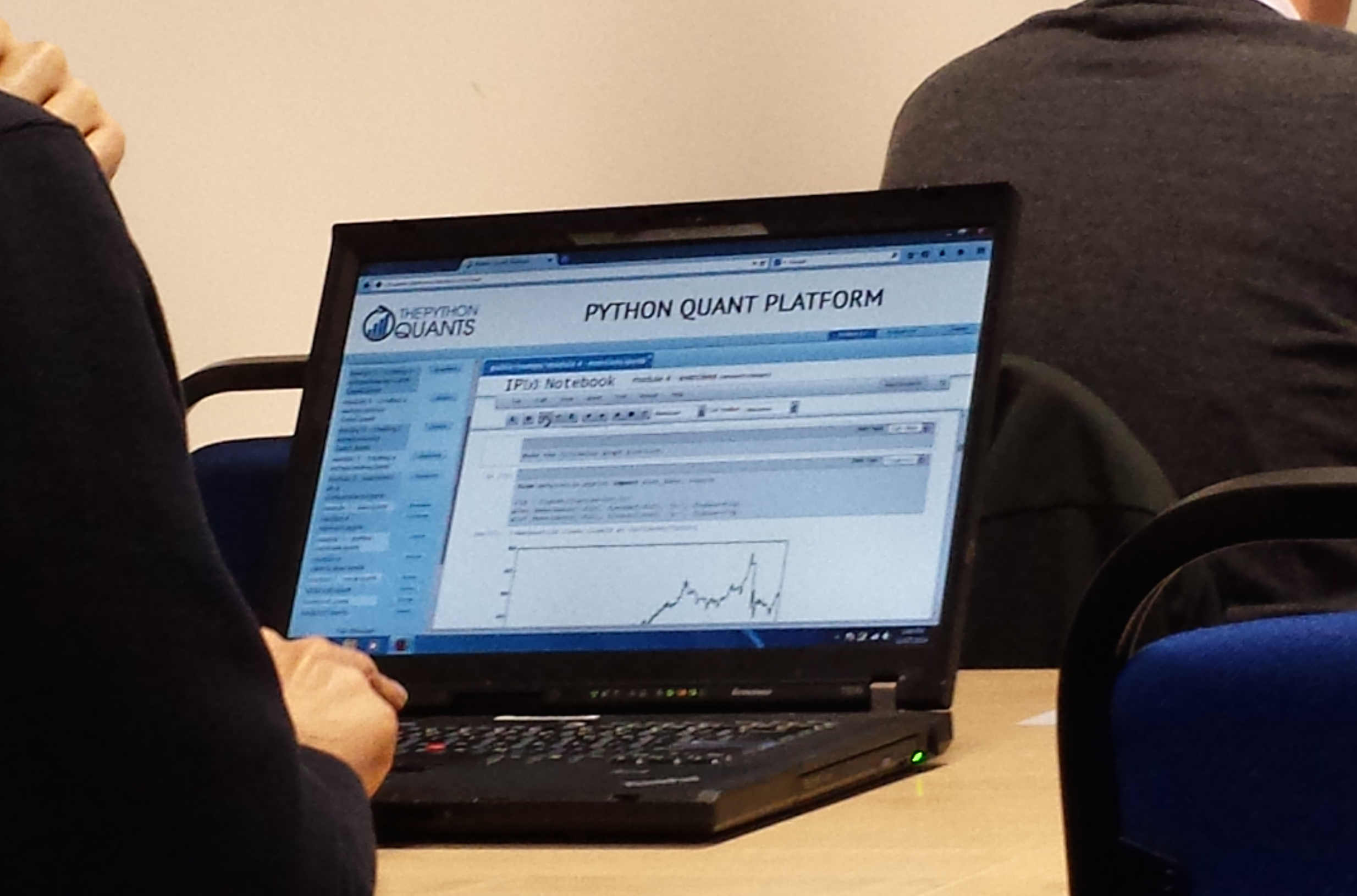
Python Quant Platform
Integrating it all and adding collaboration and scalability (http://quant-platform.com).
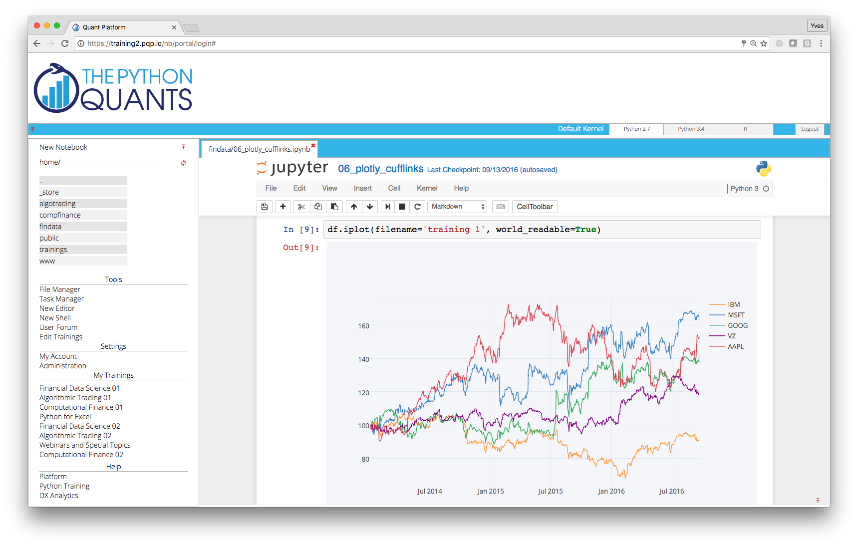
At the moment, the Python Quant Platform comprises the following components and features:
- IPython Notebook: interactive data and financial analytics in the browser with full Python integration and much more (cf. IPython home page).
- IPython Shell, Python Shell, System Shell: all you typically do on the (local or remote) system shell (Vim, Git, file operations, etc.)
- Anaconda Python Distribution: complete Python stack for financial, scientific and data analytics workflows/applications (cf. Anaconda page); you can easily switch between Python 2.7 and 3.4.
- R Stack: for statistical analyses, integrated via
rpy2and IPython Notebook - Julia: the "high-level, high-performance dynamic programming language for technical computing"
- DX Analytics: our library for advanced financial and derivatives analytics with Python based on Monte Carlo simulation.
- File Manager: a GUI-based File Manager to upload, download, copy, remove, rename files on the platform.
- Chat/Forum: there is a simple chat/forum application available via which you can share thoughts, documents and more.
- Collaboration: the platform features user/group administration as well as file sharing via public folders.
- Linux Server: the platform is powered by Linux servers to which you have full shell access.
- Deployment: the platform is easily scalable since it is cloud-based and can also be easily deployed on your own servers (via Docker containers).
During the NumPy workshop on 27. November 2014 at CQF Institute ...
DX Analytics
DX Analytics is a Python library for advanced derivatives and risk analytics. Just recently open sourced (cf. http://dx-analytics.com and http://github.com/yhilpisch/dx)
Why DX Analytics? A brief History.
Important research milestones (I), from a rather personal perspective.
- Bachelier (1900) – Option Pricing with Arithmetic Brownian Motion
- Einstein (1905) – Rigorous Theory of Brownian Motion
- Samuelson (1950s) – Systematic Approaches to Option Pricing
- Black Scholes Merton (1973) – Geometric Brownian Motion, Analytical Option Pricing Formula
- Merton (1976) – Jump Diffusion, Option Pricing with Jumps
- Boyle (1977) – Monte Carlo for European options
- Cox Ross Rubinstein (1979) – Binomial Option Pricing
Important research milestones (II), from a rather personal perspective.
- Harrison Kreps Pliska (1979/1981) – General Risk-Neutral Valuation, Fundamental Theorem of Asset Pricing
- Cox Ingersoll Ross (1985) – Intertemporal General Equilibrium, Short Rates with Square-Root Diffusion
- Heston (1993) – Stochastic Volatility, Fourier-based Option Pricing
- Bates (1996) – Heston (1993) plus Merton (1976)
- Bakshi Cao Chen (1997) – Bates (1996) plus Cox Ingersoll Ross (1985)
- Carr Madan (1999) – Using Fast Fourier Transforms for Option Pricing
- Longstaff Schwartz (2001) – Monte Carlo for American Options
- Gamba (2003) – Monte Carlo for (Complex) Portfolios of Interdependent Options
DX Analytics leverages the experience of using Python for derivatives analytics since about 10 years.
- Ph.D. research – felt in love with Harrison-Kreps-Pliska general valuation approach
- Visixion (The Python Quants) foundation in 2004 – first steps with Python & Monte Carlo simulation
- DEXISION prototyping from 2007 – using Python to build the first prototype
- DEXISION analytics suite from 2009 until today – using Python and Web technologies to provide analytics as a service
- Derivatives Analytics with Python 2011-2014 – writing a book based on university lectures and Python experience (upcoming at Wiley Finance)
- Python for Finance 2013-2014 – wiriting a book teaching Python for finance (explaining basic DX architecture)
- DX Analytics since QIV 2013 – putting all lessons learned together to write a new, concise Python library
General ideas and approaches:
- general risk-neutral valuation ("Global Valuation")
- Monte Carlo simulation for valuation, Greeks
- Fourier-based formulae for calibration
- arbitrary models for stochastic processes
- single & multi risk derivatives
- free to define payoff functions (Python syntax)
- European and American exercise
- completely implemented in Python
- hardware not a limiting factor
You can register for a PQP trial (incl. DX Analytics) here http://trial.quant-platform.com or clone the Github repo from here http://github.com/yhilpisch/dx.
A Realistic Example with DX Analytics
Bringing back office simulation and risk management practices to front office analytics.
The following more realistic example illustrates that you can model, value and risk manage quite complex derivatives portfolios with DX Analytics. The example has the following characteristics:
- portfolio over 2 years
- stochastic short rate for risk-neutral discounting
- 250 risk factors (gbm, jump diffusion, stochastic volatility)
- 1,000 derivatives (call and put options, European and American exercise, random maturites)
- monthly frequency for discretization
- 1,000 paths for simulation
from dx import *
np.random.seed(10000)
%matplotlib inline
Stochastic Short Rates
Let us start by defining a stochastic discounting object (based on CIR square-root diffusion process).
mer = market_environment(name='me', pricing_date=dt.datetime(2015, 1, 1))
mer.add_constant('initial_value', 0.005)
mer.add_constant('volatility', 0.1)
mer.add_constant('kappa', 2.0)
mer.add_constant('theta', 0.03)
mer.add_constant('paths', 1000) # dummy
mer.add_constant('frequency', 'M') # dummy
mer.add_constant('starting_date', mer.pricing_date)
mer.add_constant('final_date', dt.datetime(2015, 12, 31)) # dummy
ssr = stochastic_short_rate('ssr', mer)
Some simulated short rate paths visualized.
plt.figure(figsize=(9, 5))
plt.plot(ssr.process.time_grid, ssr.process.get_instrument_values()[:, :10]);
plt.gcf().autofmt_xdate(); plt.grid()

Multiple Risk Factors
The example is based on a multiple, correlated risk factors (based on geomtetric Brownian motion, jump diffusion or stachastic volatility models). The basic assumptions.
# market environments
me = market_environment('gbm', dt.datetime(2015, 1, 1))
# geometric Brownian motion
me.add_constant('initial_value', 36.)
me.add_constant('volatility', 0.2)
me.add_constant('currency', 'EUR')
In addition to the input parameters of the geometric Brownian motion, we also need the following for the jump diffusions and stochastic volatility models.
# jump diffusion
me.add_constant('lambda', 0.4)
me.add_constant('mu', -0.4)
me.add_constant('delta', 0.2)
# stochastic volatility
me.add_constant('kappa', 2.0)
me.add_constant('theta', 0.3)
me.add_constant('vol_vol', 0.5)
me.add_constant('rho', -0.5)
For the portfolio valuation we also need a valuation environment.
# valuation environment
val_env = market_environment('val_env', dt.datetime(2015, 1, 1))
val_env.add_constant('paths', 1000)
val_env.add_constant('frequency', 'M')
val_env.add_curve('discount_curve', ssr)
val_env.add_constant('starting_date', dt.datetime(2015, 1, 1))
val_env.add_constant('final_date', dt.datetime(2016, 12, 31))
# add valuation environment to market environments
me.add_environment(val_env)
We generate a large number of risk factors (with some random parameter values).
no = 250
risk_factors = {}
for rf in range(no):
    # random model choice
    sm = np.random.choice(['gbm', 'jd', 'sv'])
    key = '%3d_%s' % (rf + 1, sm)
    risk_factors[key] = market_environment(key, me.pricing_date)
    risk_factors[key].add_environment(me)
    # random initial_value
    risk_factors[key].add_constant('initial_value',
                                    np.random.random() * 40. + 20.)
    # radnom volatility
    risk_factors[key].add_constant('volatility',
                                    np.random.random() * 0.6 + 0.05)
    # the simulation model to choose
    risk_factors[key].add_constant('model', sm)
Correlations are also randomly chosen.
correlations = []
keys = sorted(risk_factors.keys())
for key in keys[1:]:
    correlations.append([keys[0], key, np.random.choice([-0.05, 0.0, 0.05])])
correlations[:3]
Options Modeling
We model a certain number of derivative instruments with the following major assumptions.
me_option = market_environment('option', me.pricing_date)
# choose from a set of maturity dates (month ends)
maturities = pd.date_range(start=me.pricing_date,
                           end=val_env.get_constant('final_date'),
                           freq='M').to_pydatetime()
me_option.add_constant('maturity', np.random.choice(maturities))
me_option.add_constant('currency', 'EUR')
me_option.add_environment(val_env)
Portfolio Modeling
The derivatives_portfolio object we compose consists of a large number derivatives positions. Each option differs with respect to the strike and the risk factor it is dependent on.
positions = {}
for i in range(4 * no):
    ot = np.random.choice(['am_put', 'eur_call'])
    if ot == 'am_put':
        otype = 'American single'
        payoff_func = 'np.maximum(%5.3f - instrument_values, 0)'
    else:
        otype = 'European single'
        payoff_func = 'np.maximum(maturity_value - %5.3f, 0)'
    # random strike
    strike = np.random.randint(36, 40)
    underlying = sorted(risk_factors.keys())[(i + no) % no]
    positions[i] = derivatives_position(
                        name='option_pos_%d' % strike,
                        quantity=np.random.randint(1, 10),
                        underlyings=[underlying],
                        mar_env=me_option,
                        otype=otype,
        payoff_func=payoff_func % strike)
# number of derivivatives positions
len(positions)
Portfolio Valuation
All is together to define the derivatives portfolio.
port_sequ = derivatives_portfolio(
                name='portfolio',
                positions=positions,
                val_env=val_env,
                risk_factors=risk_factors,
                correlations=correlations,
                parallel=False)  # sequential calculation
The correlation matrix illstrates the market complexity.
port_sequ.val_env.get_list('correlation_matrix')
The call of the get_values method to value all instruments.
%time res = port_sequ.get_statistics(fixed_seed=True)
The resulting table with the results.
res.set_index('position', inplace=False)
Single Option Valuation
We take out a single option from the portfolio and have a closer look.
option = port_sequ.valuation_objects[5]
option
A plot of ten paths of the underlying risk factor.
option.underlying
paths = option.underlying.get_instrument_values()[:, :10]
plt.figure(figsize=(9, 5)), plt.grid()
plt.plot(option.underlying.time_grid, paths, 'b')
plt.ylabel('risk factor level');

Valuation of the option and Greeks.
option.present_value()
option.delta()
option.vega()
Deriving values, deltas and vegas for different initial values.
%%time
S0 = option.underlying.initial_value
s_list = np.arange(S0 - 8, S0 + 8.1, 2.)
pv = []; de = []; ve = []
for s in s_list:
    option.update(s)
    pv.append(option.present_value())
    de.append(option.delta(.5))
    ve.append(option.vega(0.2))
Plotting the results.
plot_option_stats(s_list, pv, de, ve)

Risk Analysis
Full distribution of portfolio present values illustrated via histogram.
%time pvs = port_sequ.get_present_values()
plt.figure(figsize=(9, 6)); plt.hist(pvs, bins=30);
plt.xlabel('portfolio present values');plt.ylabel('frequency'); plt.grid()

Some statistics via pandas.
pdf = pd.DataFrame(pvs, columns=['values'])
pdf.describe()
The delta risk (sensitivities) report.
%%time
deltas = port_sequ.get_port_risk(Greek='Delta', fixed_seed=True, step=0.2,
                                       risk_factors=risk_factors.keys()[:4])
risk_report(deltas)
The vega risk (sensitivities) report.
%%time
vegas = port_sequ.get_port_risk(Greek='Vega', fixed_seed=True, step=0.2,
                                      risk_factors=risk_factors.keys()[:4])
risk_report(vegas)
Visualization of Selected Results
Selected results visualized.
res[['pos_value', 'pos_delta', 'pos_vega']].hist(bins=30, figsize=(9, 6))
plt.ylabel('frequency')

Sample paths for three underlyings.
paths_0 = port_sequ.underlying_objects.values()[0]
paths_0.generate_paths()
paths_1 = port_sequ.underlying_objects.values()[1]
paths_1.generate_paths()
paths_2 = port_sequ.underlying_objects.values()[2]
paths_2.generate_paths()
An the resulting plot.
pa = 5; plt.figure(figsize=(10, 6))
plt.plot(port_sequ.time_grid, paths_0.instrument_values[:, :pa], 'b');
plt.plot(port_sequ.time_grid, paths_1.instrument_values[:, :pa], 'r.-');
plt.plot(port_sequ.time_grid, paths_2.instrument_values[:, :pa], 'g-.', lw=2.5);
print 'Paths for %s (blue)' % paths_0.name
print 'Paths for %s (red)' % paths_1.name
print 'Paths for %s (green)' % paths_2.name; plt.grid()
plt.ylabel('risk factor level'); plt.gcf().autofmt_xdate()

Books
By others:
- Python for Financial Modelling @ Wiley Finance (2009)
- Python for Finance @ Packt Publishing (2014)
By myself:
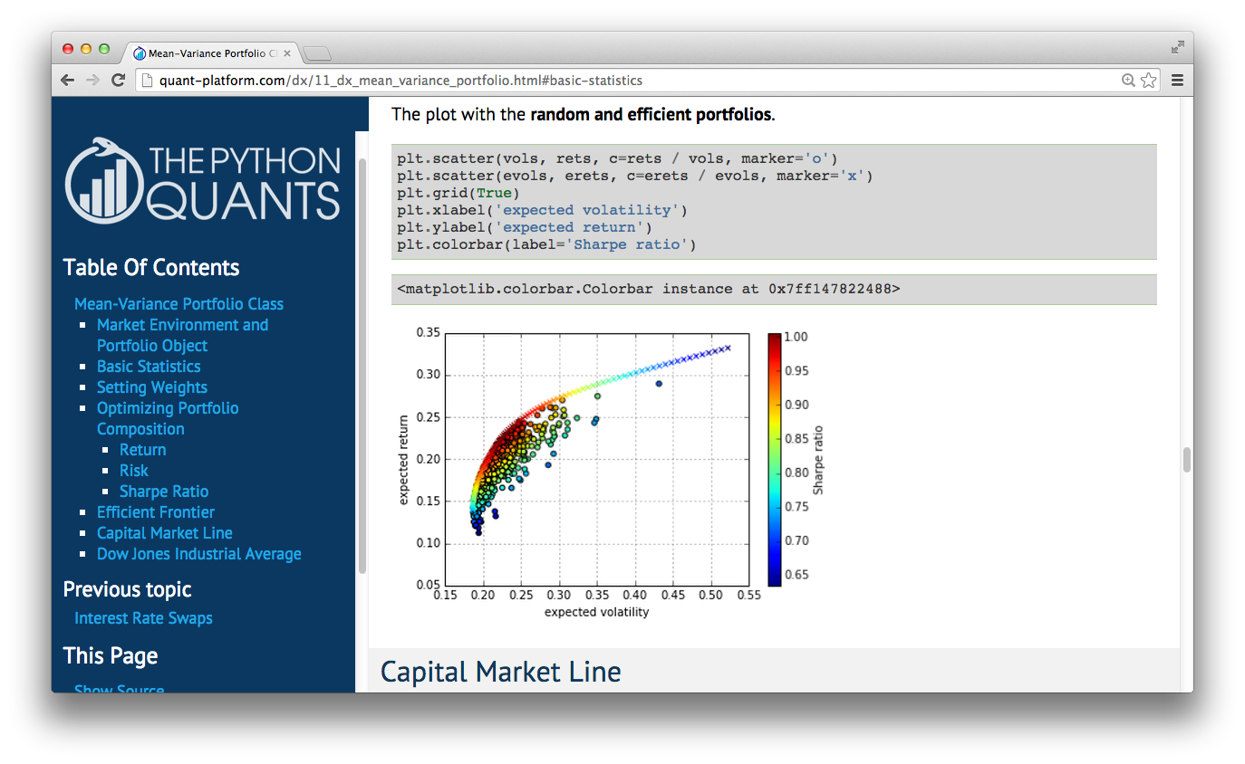
- Python for Finance – Analyze Big Financial Data @ O'Reilly (2014)
- Derivatives Analytics with Python @ Wiley Finance (2015)
Available as ebook and from December 2015 as print version.
Forthcoming 2015 at Wiley Finance ...
Meetups
For Python Quants Conference
- 1st conference in New York City on 14. March 2014
- 2nd conference in London on 28. November 2014
- 3rd conference planned for QI 2015 in Asia (eg Shanghai)
Final Thoughts
My wish for Python in the future: to become THE glue language and platform for
- data analytics
- financial analytics (derivatives, risk)
- development efforts in general
- performance technologies
- science and the technology world
- ...
Contact us
Please contact us if you have any questions or want to get involved in our Python community events.
![]()
Python Quant Platform | http://quant-platform.com
Derivatives Analytics with Python | Derivatives Analytics @ Wiley Finance
Python for Finance | Python for Finance @ O'Reilly