![]()
Volatility, Variance & Python
Exercises in Computational Finance
Yves Hilpisch
The Python Quants GmbH
10th Fixed Income Conference, Barcelona, 26. September 2014
About Me
- Founder and MD of The Python Quants GmbH
- Lecturer Mathematical Finance at Saarland University
- Co-organizer of "For Python Quants" conference in New York
- Organizer of "Python for Quant Finance" meetup in London
- Organizer of "Python for Big Data Analytics" meetup in Berlin
- Book (2015) "Derivatives Analytics with Python", Wiley Finance
- Book (2014) "Python for Finance", O'Reilly
- Dr.rer.pol in Mathematical Finance
- Graduate in Business Administration
- Martial Arts Practitioner and Fan
See www.hilpisch.com.
The Python Quants
- The Python Quants GmbH, Germany
- The Python Quants LLC., New York City
- Consulting, Development & Training
- Python and Quantitative Finance
- Python Quant Platform http://quant-platform.com
- DEXISION – GUI-based Financial Engineering www.dexision.com
- DX Analytics – Python-based derivatives analytics library
Agenda
This talk/tutorial is about new approaches for the marketing and modelling of listed volatility and variance products. The focus lies on the VSTOXX volatility index and related derivatives as well as on the just launched Variance Futures by Eurex. Topics include:
- Derivatives Analytics
- DX Analytics
- VSTOXX Advanced Services (static)
- Python Quant Platform
- VSTOXX Advanced Services (interactive)
- VSTOXX Options Pricing
- Variance Advanced Services
Derivatives Analytics
Historical Milestones
Important Milestones (I), from a rather personal perspective.
- Bachelier (1900) – Option Pricing with Arithmetic Brownian Motion
- Einstein (1905) – Rigorous Theory of Brownian Motion
- Samuelson (1950s) – Systematic Approaches to Option Pricing
- Black Scholes Merton (1973) – Geometric Brownian Motion, Analytical Option Pricing Formula
- Merton (1976) – Jump Diffusion, Option Pricing with Jumps
- Boyle (1977) – Monte Carlo for European options
- Cox Ross Rubinstein (1979) – Binomial Option Pricing
Important Milestones (II), from a rather personal perspective.
- Harrison Kreps Pliska (1979/1981) – General Risk-Neutral Valuation, Fundamental Theorem of Asset Pricing
- Cox Ingersoll Ross (1985) – Intertemporal General Equilibrium, Short Rates with Square-Root Diffusion
- Heston (1993) – Stochastic Volatility, Fourier-based Option Pricing
- Bates (1996) – Heston (1993) plus Merton (1976)
- Gruenbichler Longstaff (1996) – Volatility Futures and Options Pricing
- Bakshi Cao Chen (1997) – Bates (1996) plus Cox Ingersoll Ross (1985)
- Carr Madan (1999) – Using Fast Fourier Transforms for Option Pricing
- Longstaff Schwartz (2001) – Monte Carlo for American Options
- Gamba (2003) – Monte Carlo for (Complex) Portfolios of Interdependent Options
Anlytical Formulae vs. Numerical Methods
Potential problems with analytical formulae for pricing/valuation:
- black box
- limited/specific use cases
- no consistent value aggregation
- no consistent risk aggregation/netting
- no full distribution (only point estimate)
- no incorporation of correlation
Sometimes significant advantages of analytical formulae for pricing/valuation:
- often easy to understand and apply (without knowing about the theory behind it)
- in general high speed for numerical evaluations
- low technical requirements (computing power, memory)
- implementable on "every" machine
- easy testing/maintenance of implemented formulae
Alleged drawbacks of alternative numerical methods (such as simulation):
- compute intensive
- memory intensive
- accuracy issues (e.g. convergence)
- conceptual problems (e.g. American exercise)
- implementation issues (e.g. algorithms, performance, memory)
- testing/maintenance issues (e.g. test coverage)
On the other hand, many benefits from numerical methods (such as simulation):
- highly flexible and powerful (any model, any derivative, any portfolio)
- full distributional view (values, risk, portfolio)
- consistent value aggregation (path-wise)
- consistent risk measures (full distribution)
- consistent estimation of netting effects (path-wise)
- consistent incorporation of (time-varying) correlations
- full graphical analysis (no black boxes or corners)
Avances in Technology
Not too long ago ...
- desktops, notebooks (maybe connected via Internet)
- dedicated, individual servers (if at all)
- single or few cores, little memory
- low level programming languages (C, Fortran)
- mainly sequential execution of code
- (prohibitively) high costs for high performance
Today, we are a bit more lucky ...
- desktops, notebooks as workstations
- Cloud-based computing (with custom nodes)
- many cores, large memory, powerful GPUs
- high level programming languages (Python)
- on demand scalability and parallelization
- low (variable) costs for large machines & high performance
DX Analytics
A Pythonic Library for Simulation-Based Derivatives Analytics developed and maintained by The Python Quants.
Overview
General ideas and approaches:
- general risk-neutral valuation ("Global Valuation")
- Monte Carlo simulation for valuation, Greeks
- Fourier-based formulae for calibration
- arbitrary models for stochastic processes
- single & multi risk derivatives
- European and American exercise
- completely implemented in Python
- hardware not a limiting factor
Global Valuation at its core:
- non-redundant modeling (e.g. of risk factors)
- consistent simulation (e.g. given correlations)
- consistent value and risk aggregation
- single positions or consistent portfolio view
Python specifics:
- heavy use of classes and object orientation
- NumPy ndarray class and pandas DataFrame class for numerical data
- Python dictionaries (mainly) for meta data
American Put Option
We model and value a simple American put option. First the underlying.
import dx
import numpy as np
import datetime as dt
r = dx.constant_short_rate('short_rate', 0.06)
me = dx.market_environment('gbm', dt.datetime(2015, 1, 1))
me.add_constant('initial_value', 36.)
me.add_constant('volatility', 0.2)
me.add_constant('currency', 'USD')  # currency
me.add_constant('frequency', 'W')  # pandas date_range frequency string
me.add_constant('paths', 50000)  # number of paths
me.add_constant('final_date', dt.datetime(2015, 12, 31))
me.add_curve('discount_curve', r)
gbm = dx.geometric_brownian_motion('gbm', me)  # simulation object
gbm.generate_paths()
A visualization of the first ten simulated paths.
import matplotlib.pyplot as plt
%matplotlib inline
fig = plt.figure(figsize=(9, 5))
plt.plot(gbm.time_grid, gbm.get_instrument_values()[:, :10]);
plt.grid(True); fig.autofmt_xdate()

Second, the American put option.
me_put = dx.market_environment('put', gbm.pricing_date)
me_put.add_constant('maturity', gbm.final_date)
me_put.add_constant('strike', 40.)
me_put.add_constant('currency', 'USD')
put = dx.valuation_mcs_american_single(
        'put', gbm, me_put,
        payoff_func='np.maximum(strike - instrument_values, 0)')
Valuation and Greeks for the American put.
put.present_value()
put.delta()
put.vega()
Some sensitivities of the American put (I).
%%time
s_list = np.arange(32., 50.1, 2.)
pv = []; de = []; ve = []
for s in s_list:
    put.update(initial_value=s)
    pv.append(put.present_value())
    de.append(put.delta())
    ve.append(put.vega())
put.update(initial_value=36.)
Some sensitivities of the American put (II).
dx.plot_option_stats(s_list, pv, de, ve)

European Maximum Call Option
Now a more complex, two risk factor European option.
%run dx_example.py
  # sets up market environments
  # and defines derivative instrument
max_call.payoff_func
  # payoff of a maximum call option
  # on two underlyings (European exercise)
We are going to generate a Vega surface for one risk factor with respect to the initial values of both risk factors.
asset_1 = np.arange(28., 46.1, 2.)
asset_2 = asset_1
a_1, a_2 = np.meshgrid(asset_1, asset_2)
value = np.zeros_like(a_1)
%%time
vega_gbm = np.zeros_like(a_1)
for i in range(np.shape(vega_gbm)[0]):
    for j in range(np.shape(vega_gbm)[1]):
        max_call.update('gbm', initial_value=a_1[i, j])
        max_call.update('jd', initial_value=a_2[i, j])
        vega_gbm[i, j] = max_call.vega('gbm')
The results visualized.
dx.plot_greeks_3d([a_1, a_2, vega_gbm], ['gbm', 'jd', 'vega gbm'])
  # Vega surface plot

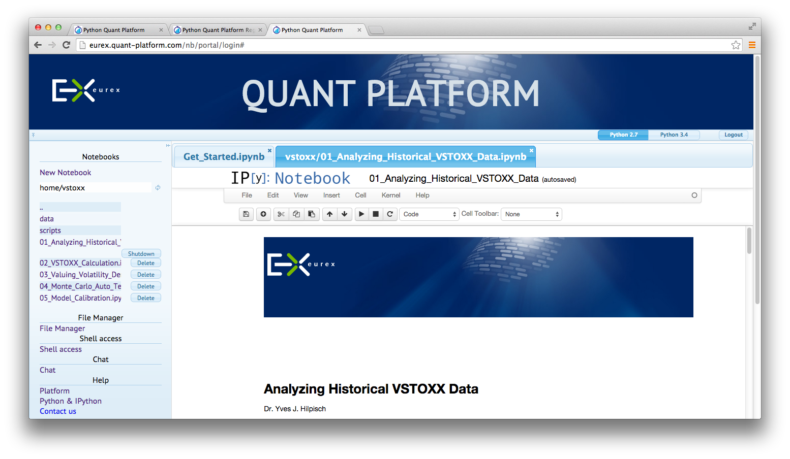
VSTOXX Advanced Services (Static)
In June 2013, Eurex launched the VSTOXX Advanced Services, a series of Python-based tutorials about the VSTOXX and related derivatives. Contents covered:
- Python Preliminaries
- Analyzing Historical VSTOXX Data
- Calculating the VSTOXX Index
- Valuing Volatility Derivatives
- Automated Monte Carlo Tests
- Calibration of the Pricing Model
- Backtesting of VSTOXX Strategies
See http://www.eurexchange.com/vstoxx/ and http://www.eurexchange.com/vstoxx/app2/.
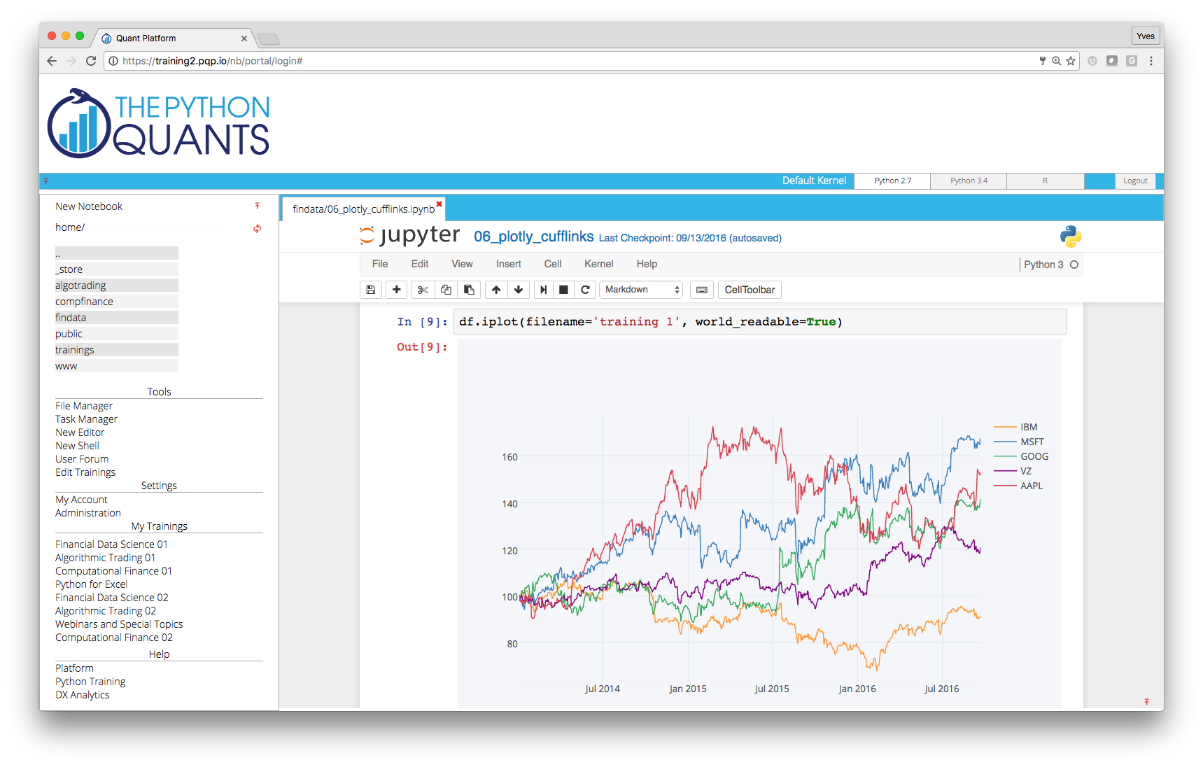
Python Quant Platform
The Python Quant Platform is developed and maintained by The Python Quants. It offers Web-/browser-based data and financial analytics for individuals, teams and organizations. Free registrations are possible under http://trial.quant-platform.com.
You can freely choose your user name and password. You can then login under http://analytics.quant-platform.com, using trial as company in combination with your user name and password.
At the moment, the Python Quant Platform comprises the following components and features:
- IPython Notebook: interactive data and financial analytics in the browser with full Python integration and much more (cf. IPython home page).
- Anaconda Python Distribution: complete Python stack for financial, scientific and data analytics workflows/applications (cf. Anaconda page); you can easily switch between Python 2.7 and 3.4.
- DX Analytics: our library for advanced financial and derivatives analytics with Python based on Monte Carlo simulation.
- File Manager: a GUI-based File Manager to upload, download, copy, remove, rename files on the platform.
- Chat/Forum: there is a simple chat/forum application available via which you can share thoughts, documents and more.
- Collaboration: the platform features user/group administration as well as file sharing via public folders.
- Linux Server: the platform is powered by Linux servers to which you have full shell access (eg for IPython shell, Vim editing, Git integration).
- Deployment: the platform is easily scalable since it is cloud-based and can also be easily deployed on your own servers (via Docker containers).
IPython Notebook provides a unified analytics environment for a couple of (domain specific) languages, like R.
%load_ext rpy2.ipython
X = np.arange(100)
Y = 2 * X + 5 + 2 * np.random.standard_normal(len(X))
%Rpush X Y
Plotting with R from within IPython.
%R plot(X, Y, pch=19, col='blue'); grid(); title("R Plot with IPython")

Doing statistics with R.
%R print(summary(lm(Y~X)))
Pulling data from R to Python.
%R c = coef(lm(Y~X))
%Rpull c
c
VSTOXX Advanced Services (Interactive)
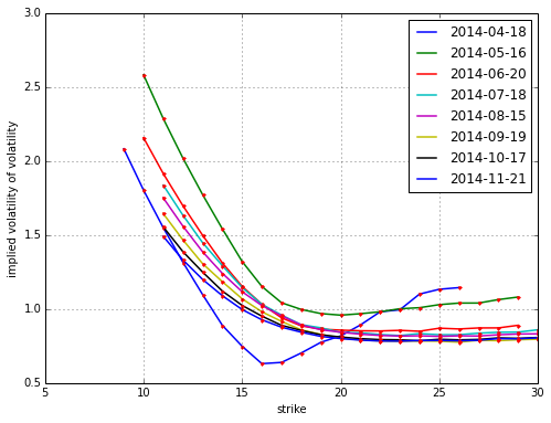
VSTOXX Options Pricing
Vol-Vol Surface
VSTOXX implied vol-vol on 28. Dezember 2012.
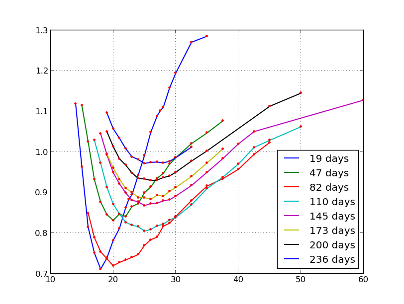
VSTOXX implied vol-vol on 31. March 2014.
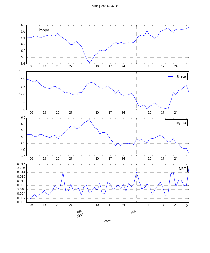
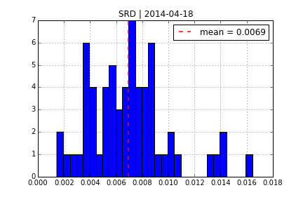
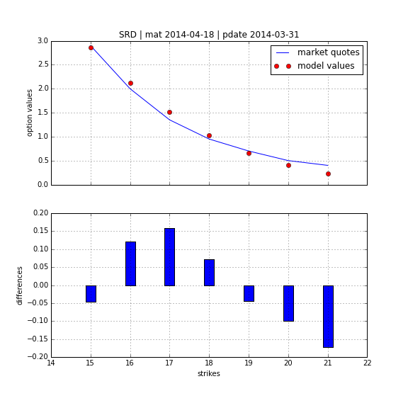
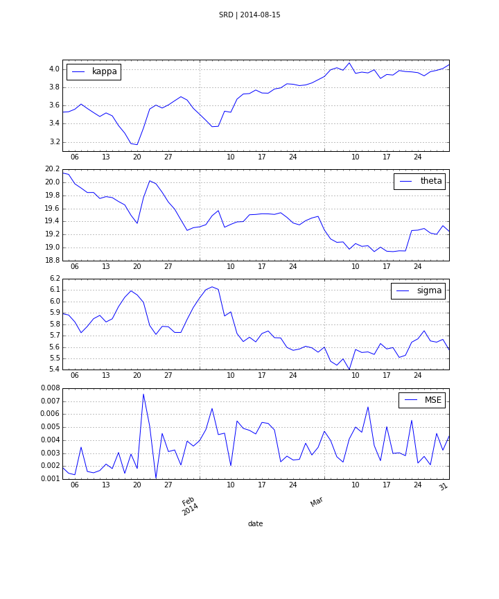
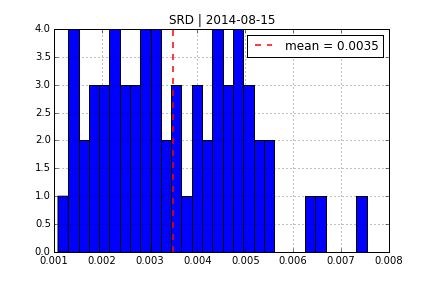
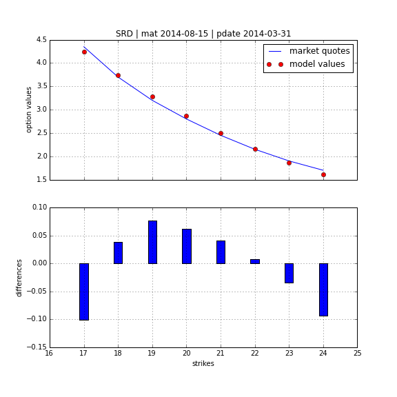
Square-Root Diffusion
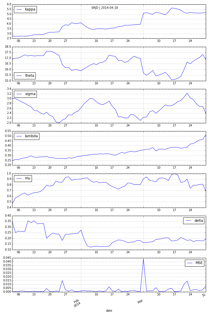
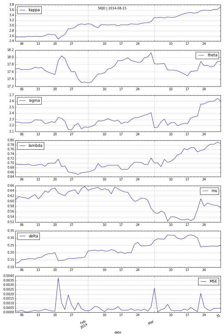
One of the early models for volatility option pricing has been the square-root diffusion process (SRD) as proposed by Gruenbichler Longstaff (1996):
$$ dv_{t}=\kappa (\theta -v_{t})dt+\sigma \sqrt{v_{t}}dZ_{t} $$
The meaning of the variables and parameters is
- $v_{t}$ volatility index level at date $t$
- $\kappa$ speed of adjustment of $v_{t}$ to ...
- $\theta$, the long-term mean of the index
- $\sigma$ volatility coefficient of the index level
- $Z_{t}$ standard Brownian motion
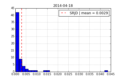
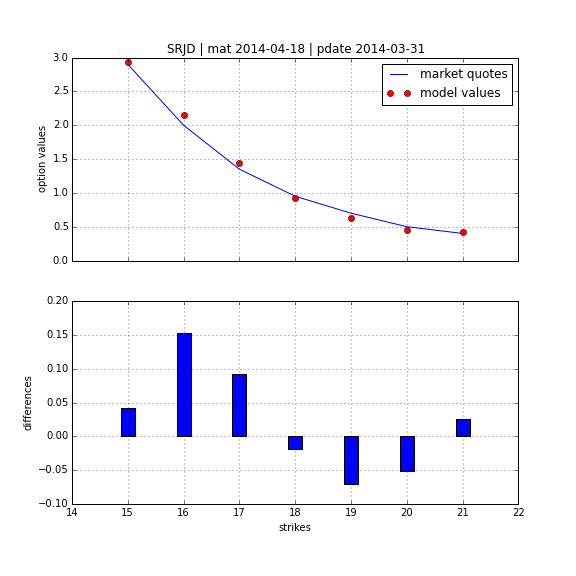
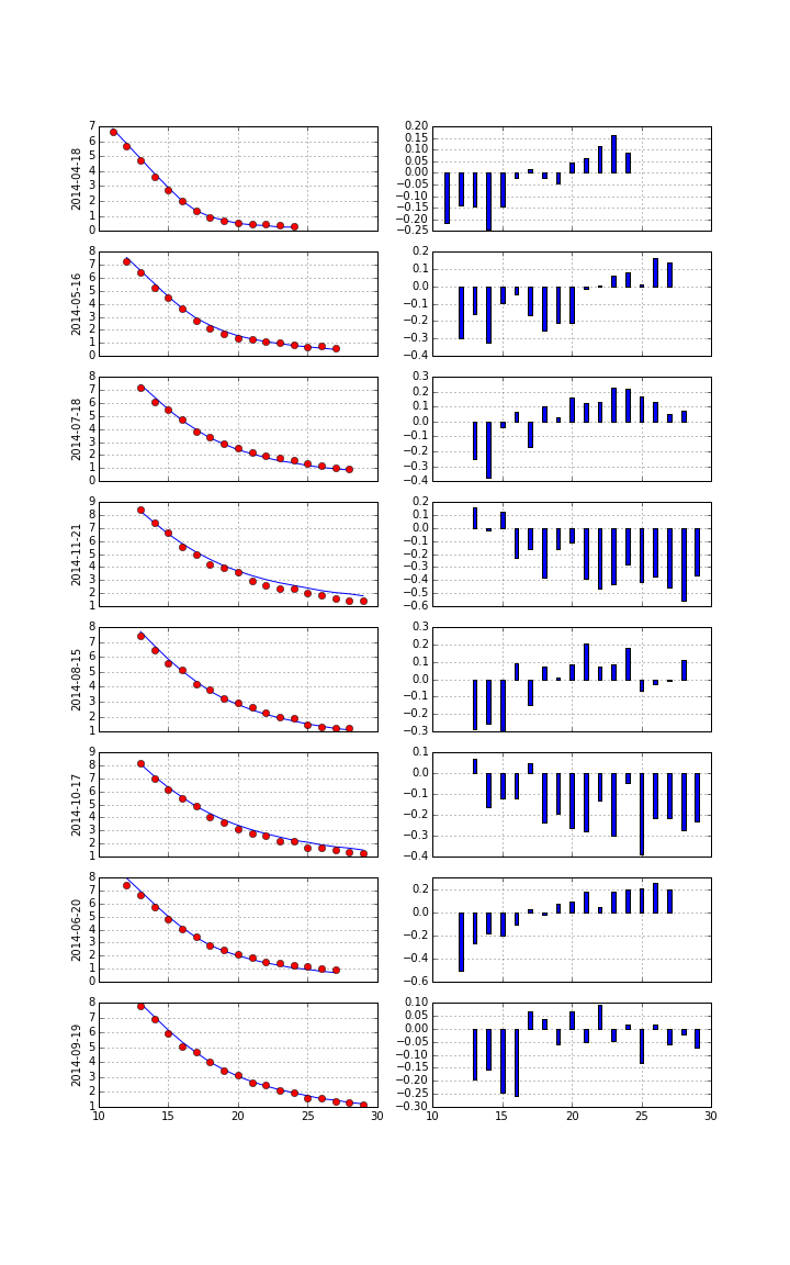
Using DX Analytics, we calibrate the SRD model to European call options on the VSTOXX. The time series data is from QI of 2014. We calibrate to 2 maturities:
- April 2014 (shortest one with data available throughout)
- August 2014 (longest one with data available throughout)
Square-Root Jump Diffusion
To better account for the vol-vol smile implied in volatility option prices as well as for jumps, we add a log-normal jump compnent to the SRD process to end up with a square-root jump diffusion (SRJD):
$$ dv_{t}=\kappa (\theta -v_{t})dt+\sigma \sqrt{v_{t}}dZ_{t} + J_{t} v_{t} dN_{t} -r_{J}dt $$
- $J_{t}$ jump at date $t$ with distribution ...
- ... $\log(1+J_{t})\approx \mathbf{N}\left(\log(1+\mu)-\frac{\delta^{2}}{2},\delta^{2}\right)$
- $\mathbf{N}$ cumulative distribution function of a standard normal random variable
- $N_{t}$ Poisson process with intensity $\lambda$
- $r_{J}\equiv \lambda \cdot \left(e^{\mu + \delta^{2}/2}-1\right)$ drift correction for jump
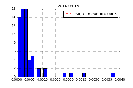
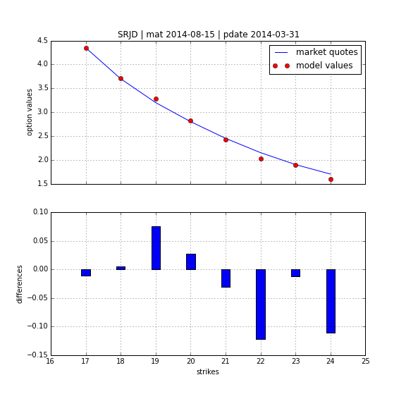
Square Root Jump Diffusion Plus
Taking the term structure, i.e. futures prices, into account and calibrating the model to multiple maturities simulataneously. Cf. CIR+ model by Brigo Mercurio (2001).
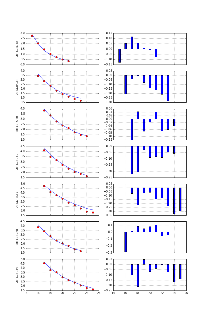
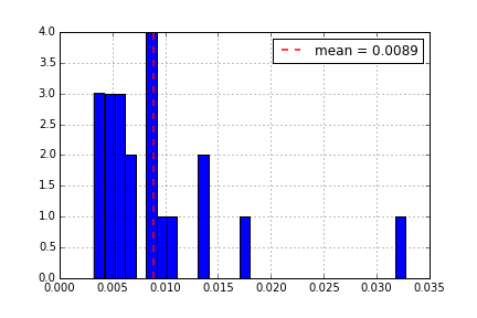
Calibration over all maturities with +/-40% otm/itm options (total of 129 options).
Variance Advanced Services
To be launched rather soon with the following topics covered:
- Realized Variance and Variance Swaps
- Model-Free Replication of Variance
- Variance Futures at Eurex
- Trading and Settlement
- Backtesting Data
- Quant Platform
![]()
Python Quant Platform | http://quant-platform.com
Derivatives Analytics with Python | Derivatives Analytics @ Wiley Finance
Python for Finance | Python for Finance @ O'Reilly