Computational Finance — Why Python is Taking Over

A Subjective and Biased Overview

Dr. Yves J. Hilpisch | The Python Quants GmbH

team@tpq.io | www.quant-platform.com

Quant Insights, London, 30. October 2015

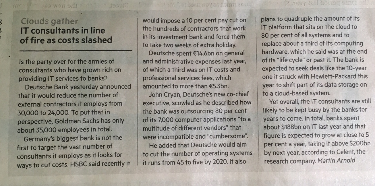
State of Technology in Banking¶

From the Financial Times, 30. October 2015.

The Python Language¶

Black-Scholes-Merton (1973) SDE of geometric Brownian motion.

$$ dS_t = rS_tdt + \sigma S_t dZ_t $$

Monte Carlo simulation: draw $I$ standard normally distributed random numbers $z_t^i$ and apply them to the following by Euler disctretization scheme to simulate $I$ end values of the GBM:

$$ S_{T} = S_0 \exp \left(\left( r - \frac{1}{2} \sigma^2\right) T + \sigma \sqrt{T} z_T \right) $$

Latex description of Euler discretization.

S_T = S_0 \exp (( r - 0.5 \sigma^2 ) T + \sigma \sqrt{T} z_T)

Python implementation of algorithm.

In [2]:

from pylab import *
S_0 = 100.; r = 0.01; T = 0.5; sigma = 0.2
z_T = standard_normal(10000)

In [3]:

S_T = S_0 * exp((r - 0.5 * sigma ** 2) * T + sigma * sqrt(T) * z_T)

Again, Latex for comparison:

S_T = S_0 \exp (( r - 0.5 \sigma^2 ) T + \sigma \sqrt{T} z_T)

Interactive visualization of simulation results.

In [4]:

%matplotlib inline
pyfig = figure()
hist(S_T, bins=40);

The Python Ecosystem¶

IPython & Jupyter (interactive prototyping/analytics in the browser)
NumPy (fast, vectorized array operations)
SciPy (collection of scientific classes/functions)
pandas (times series and tabular data)
ibis (Pythonic interaction with eg relational databases)
PyTables (hardware-bound IO operations)
TsTables (high performance tick data storage/retrieval)
scikit-learn (machine learning algorithms)
statsmodels (statistical classes/functions)
xlwings (Python-Excel integration)

Financial Libraries¶

By others:

zipline (backtesting of trading algos)
PyThalesians (data, backtesting, trading)
Pyfolio (portfolio management, Quantopian)
matplotlib.finance (financial plots)
Python wrappers (QuantLib)

By us:

DEXISION – GUI-based financial engineering
DX Analytics – global valuation of multi-risk derivatives and portfolios

Example: DX Analytics — Simple

DX Analytics is a Python library for advanced financial and derivatives analytics written by The Python Quants. It is particularly suited to model multi-risk derivatives and to do a consistent valuation of portfolios of complex derivatives. It mainly uses Monte Carlo simulation since it is the only numerical method capable of valuing and risk managing complex, multi-risk derivatives books.

An example with an European maximum call option on two underlyings.

In [5]:

%%time
import dx
%run dx_example.py
  # sets up market environments
  # and defines derivative instrument
  # calculates a number of numerical results

CPU times: user 5.87 s, sys: 422 ms, total: 6.29 s
Wall time: 7.01 s

In [6]:

max_call.payoff_func
  # payoff of a maximum call option
  # on two underlyings (European exercise)

Out[6]:

"np.maximum(np.maximum(maturity_value['gbm'], maturity_value['jd']) - 34., 0)"

In [7]:

max_call.vega('jd')
  # numerical Vega with respect
  # to one risk factor

Out[7]:

0.7999999999999119

A Vega surface for one risk factor with respect to the initial values of both risk factors.

In [8]:

dx.plot_greeks_3d([a_1, a_2, vega_gbm], ['gbm', 'jd', 'vega gbm'])
  # Vega surface plot

Example: DX Analytics — Complex

This example values a portfolio with 50 (correlated) risk factors and 250 options (European/American exercise) via Monte Carlo simulation in risk-neutral fashion with stochastic short rates.

http://dx-analytics.com/13_dx_quite_complex_portfolios.html

APIs – Interfacing with Others

OANDA (fx/cfd trading platform)
Thomson Reuters (Python wrapper for unified API soon available)
Front Arena (scripting with Python)
Murex (scripting payoffs with Python)
...

Example: Murex¶

From http://www.risk.net:

"Murex provides a complete cross-asset and front-to-back offering for structured products, combining out-of-the box complex payoffs and models with structuring tools, and model and products catalogue extensors.

Key features include:

A wide native catalogue of exotic products and best-of-breed models, all compliant with a grid.
A generic Monte Carlo, fully compliant with graphics processing units, providing impressive performance speed-ups.
A structured trade builder to create any on-the-fly packages, persistent contracts and structured over-the-counter trades or securities – for example, warrants and bonds.
A payoff language to describe any complex exotic with an interpreted language (Python) in an unbeatable time to market, and for both revaluation and front-to-back integration."

Integration – No "Either Or" with Python

C/C++ (natively)
Julia (IPython/Jupyter)
JavaScript (IPython)
Matlab (NumPy)
R (Jupyter/rpy2)
...

Example: Statistics with R¶

We analyze the statistical correlation between the EURO STOXX 50 stock index and the VSTOXX volatility index.

First the EURO STOXX 50 data.

In [9]:

import pandas as pd
cols = ['Date', 'SX5P', 'SX5E', 'SXXP', 'SXXE',
        'SXXF', 'SXXA', 'DK5F', 'DKXF', 'DEL']
es_url = 'http://www.stoxx.com/download/historical_values/hbrbcpe.txt'
try:
    es = pd.read_csv(es_url,  # filename
                     header=None,  # ignore column names
                     index_col=0,  # index column (dates)
                     parse_dates=True,  # parse these dates
                     dayfirst=True,  # format of dates
                     skiprows=4,  # ignore these rows
                     sep=';',  # data separator
                     names=cols)  # use these column names

    # deleting the helper column
    del es['DEL']
except:
    # read stored data if there is no Internet connection
    es = pd.HDFStore('data/SX5E.h5', 'r')['SX5E']

Second, the VSTOXX data.

In [10]:

vs_url = 'http://www.stoxx.com/download/historical_values/h_vstoxx.txt'

try:
    vs = pd.read_csv(vs_url,  # filename
                     index_col=0,  # index column (dates)
                     parse_dates=True,  # parse date information
                     dayfirst=True, # day before month
                     header=2)  # header/column names
except:
    # read stored data if there is no Internet connection
    vs = pd.HDFStore('data/V2TX.h5', 'r')['V2TX']

Generating log returns with Python and pandas.

In [11]:

import numpy as np
# log returns for the major indices' time series data
datv = pd.DataFrame({'SX5E' : es['SX5E'], 'V2TX': vs['V2TX']}).dropna()
rets = np.log(datv / datv.shift(1)).dropna()
ES = rets['SX5E'].values
VS = rets['V2TX'].values

Bridging to R from within IPython Notebook and pushing Python data to the R run-time.

In [12]:

%load_ext rpy2.ipython

In [13]:

%Rpush ES VS

Plotting with R in IPython Notebook.

In [14]:

%R plot(ES, VS, pch=19, col='blue'); grid(); title("Log returns ES50 & VSTOXX")

Linear regression with R.

In [15]:

%R c = coef(lm(VS~ES))

Out[15]:

array([  9.15896671e-06,  -2.83354384e+00])

In [16]:

%R print(summary(lm(VS~ES)))

Call:
lm(formula = VS ~ ES)

Residuals:
     Min       1Q   Median       3Q      Max 
-0.32413 -0.02188 -0.00207  0.02042  0.53806 

Coefficients:
              Estimate Std. Error t value Pr(>|t|)    
(Intercept)  9.159e-06  6.038e-04   0.015    0.988    
ES          -2.834e+00  3.996e-02 -70.910   <2e-16 ***
---
Signif. codes:  0 ‘***’ 0.001 ‘**’ 0.01 ‘*’ 0.05 ‘.’ 0.1 ‘ ’ 1

Residual standard error: 0.03951 on 4281 degrees of freedom
Multiple R-squared:  0.5401,	Adjusted R-squared:   0.54 
F-statistic:  5028 on 1 and 4281 DF,  p-value: < 2.2e-16

Regression line visualized.

In [17]:

%R plot(ES, VS, pch=19, col='blue'); grid(); abline(c, col='red', lwd=5)

Pulling data from R to Python and using it.

In [18]:

%Rpull c

In [19]:

plt.figure(figsize=(10, 6))
plt.plot(ES, VS, 'b.')
plt.plot(ES, c[0] + c[1] * ES, 'r', lw=3)
plt.xlabel('ES'); plt.ylabel('VS')

Out[19]:

<matplotlib.text.Text at 0x10b7e1410>

If you want to have it nicer, interactive and embeddable anywhere – use plot.ly

In [20]:

import plotly.plotly as py
py.sign_in('Python-Demo-Account', 'gwt101uhh0')

Let us generate a plot with a bit fewer data points.

In [21]:

pyfig = plt.figure(figsize=(9, 6)); n = 100
plt.plot(ES[:n], VS[:n], 'b.')
plt.plot(ES[:n], c[0] + c[1] * ES[:n], 'r', lw=3)
plt.xlabel('ES'); plt.ylabel('VS')

Out[21]:

<matplotlib.text.Text at 0x110259390>

Only single line of code needed to convert matplotlib plot into interactive D3 plot.

In [22]:

py.iplot_mpl(pyfig)  # convert mpl plot into interactive D3

Out[22]:

Performance – Numerical Algorithms

Finance algorithms are loop-heavy; Python loops are slow; Python is too slow for finance.

In [23]:

def counting_py(N):
    s = 0
    for i in xrange(N):
        for j in xrange(N):
            s += int(cos(log(1)))
    return s

In [24]:

N = 2000
%time counting_py(N)
# memory efficient but slow

CPU times: user 8.19 s, sys: 75.3 ms, total: 8.27 s
Wall time: 8.66 s

Out[24]:

First approach: vectorization with NumPy.

In [25]:

%%time
from pylab import *
arr = ones((N, N))
print int(sum(cos(log(arr))))

4000000
CPU times: user 84.4 ms, sys: 45 ms, total: 129 ms
Wall time: 130 ms

In [26]:

arr.nbytes # much faster but NOT memory efficient

Out[26]:

32000000

Second approach: dynamic compiling with Numba.

In [27]:

import numba
counting_nb = numba.jit(counting_py)

In [28]:

%time counting_nb(N)
# some overhead the first time

CPU times: user 141 ms, sys: 16.8 ms, total: 158 ms
Wall time: 151 ms

Out[28]:

In [29]:

%timeit counting_nb(N)
# even faster AND memory efficient

10 loops, best of 3: 52.5 ms per loop

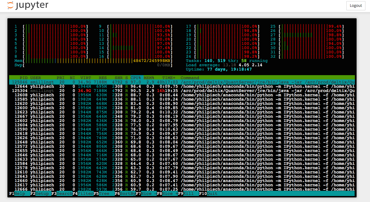
Performance – Hardware-bound IO

Hardware-bound IO operations are standard for Python.

In [30]:

%time one_gb = standard_normal((12500, 10000))
one_gb.nbytes
# a giga byte worth of data

CPU times: user 6.3 s, sys: 486 ms, total: 6.79 s
Wall time: 7.04 s

Out[30]:

1000000000

In [31]:

%time save('one_gb', one_gb)

CPU times: user 59.6 ms, sys: 2.73 s, total: 2.79 s
Wall time: 3.94 s

In [32]:

!ls -n one_gb*

-rw-r--r--  1 501  20  1000000080 Oct 30 09:30 one_gb.npy

Python Quant Platform¶

Integrating it all and adding collaboration and scalability (http://quant-platform.com).

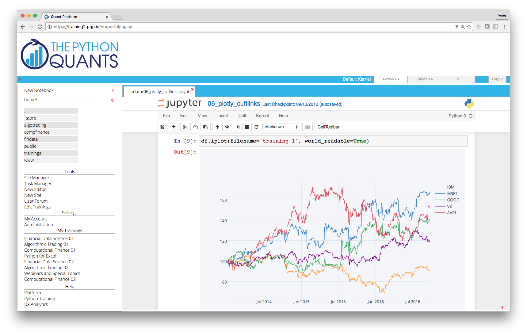
At the moment, the Python Quant Platform comprises the following components and features:

Jupyter Notebook: interactive data and financial analytics in the browser with full Python integration and much more (cf. IPython home page).
IPython Shell, Python Shell, System Shell: all you typically do on the (local or remote) system shell (Vim, Git, file operations, etc.)
Anaconda Python Distribution: complete Python stack for financial, scientific and data analytics workflows/applications (cf. Anaconda page); you can easily switch between Python 2.7 and 3.4.
R Stack: for statistical analyses, integrated via rpy2 and IPython Notebook
Julia Stack: for HPC computing "in the spirit" of Python based on LLVM
DX Analytics: our library for advanced financial and derivatives analytics with Python based on Monte Carlo simulation.
File Manager: a GUI-based File Manager to upload, download, copy, remove, rename files on the platform.
Chat/Forum: there is a simple chat/forum application available via which you can share thoughts, documents and more.
Collaboration: the platform features user/group administration as well as file sharing via public folders.
Linux Server: the platform is powered by Linux servers to which you have full shell access.
Deployment: the platform is easily scalable since it is cloud-based and can also be easily deployed on your own servers (via Docker containers).

Example: Cloud-based Analytics & Storage¶

Quant Platform/datapark.io are fully integrated with Dropbox. Use the platform as a cloud-based execution environment for code and data stored on Dropbox.

Example: Publishing Research Results on the Platform¶

In [34]:

from IPython.display import HTML
HTML('<iframe src=http://web.quant-platform.com/trial/yves/ \
      width=100% height=550></iframe>')

Out[34]:

The Large Banks¶

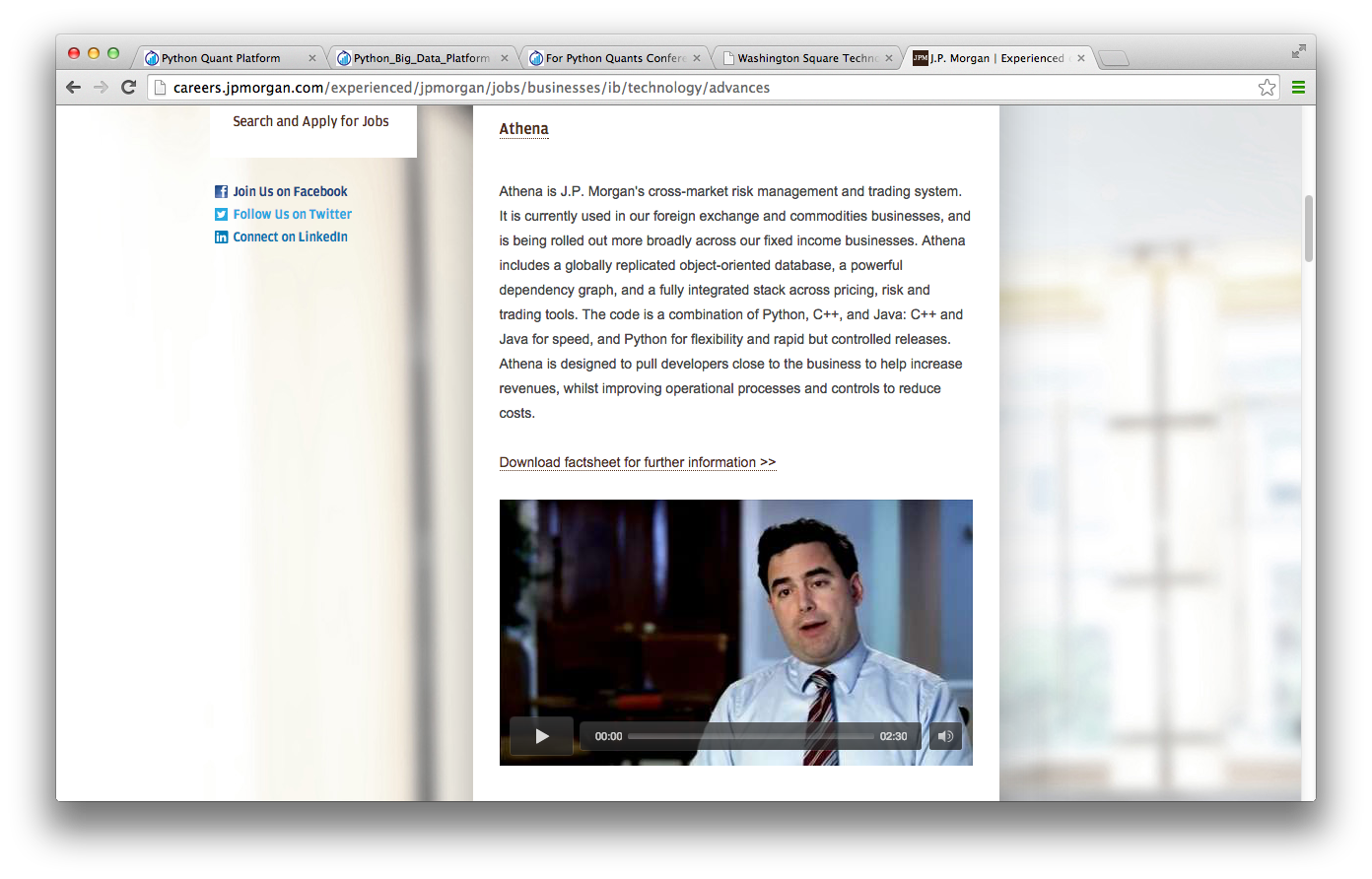
JPMorgan Chase (Athena platform)
Bank of America Merrill Lynch (Quartz platform)
Deutsche Bank (equity research)
Lloyds Bank
BNP Paribas
Nomura
...

Example: JPMorgan¶

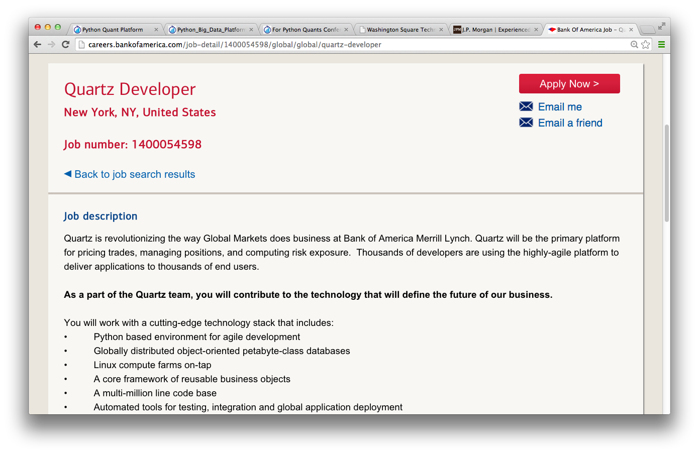
Example: Bank of America Merrill Lynch¶

The Hedge Funds¶

AQR Capital Management (origin of pandas)
Two Sigma Investments (large scale data analytics)
ARC Investments (full-fledged Python for vol trading)
...

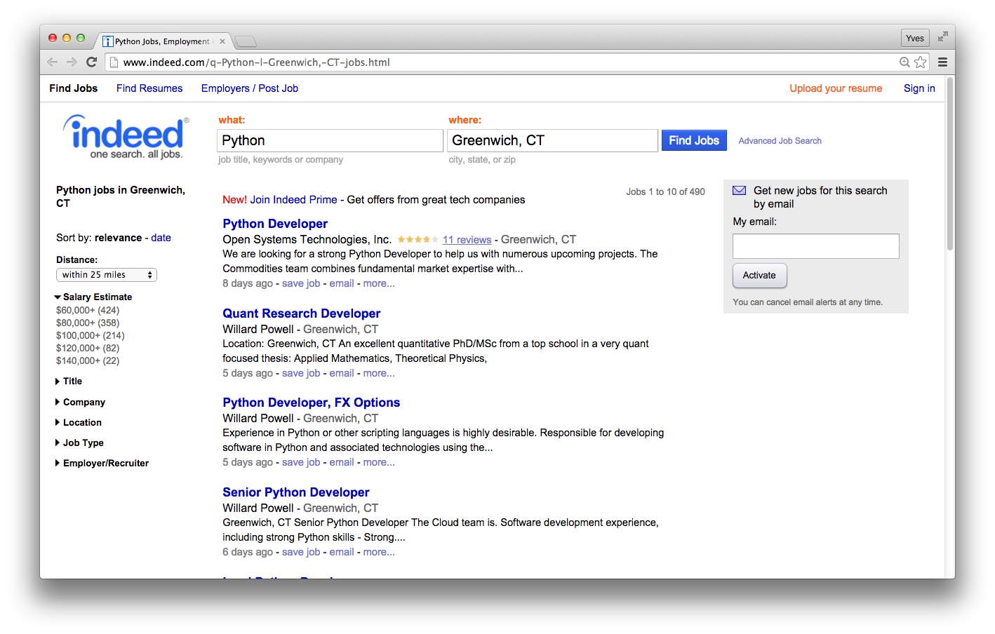
Example: Python Jobs in Greenwich (CT)¶

490 Python Jobs in Greenwich, CT – obviously a famous hedge fund place.

Innovators in the Space¶

Quantopian (algo trading & backtesting)
Washington Square Technologies (trade & risk platform)
Deutsche Boerse/Eurex (VSTOXX and Variance Advanced Services)
...

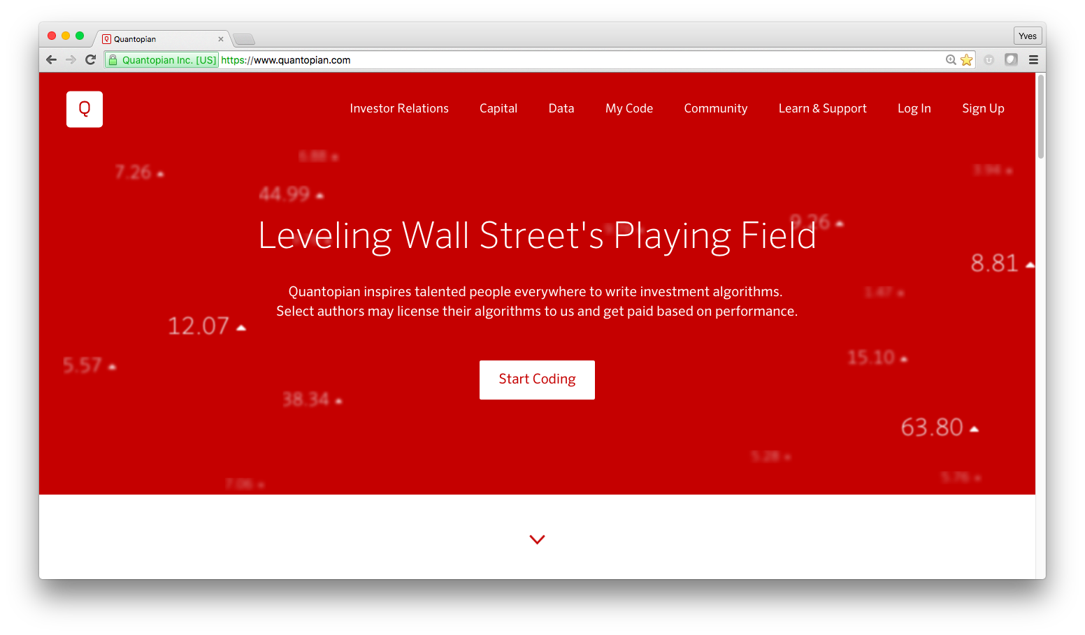
Example: Quantopian¶

Automated Trading powerd by Python.

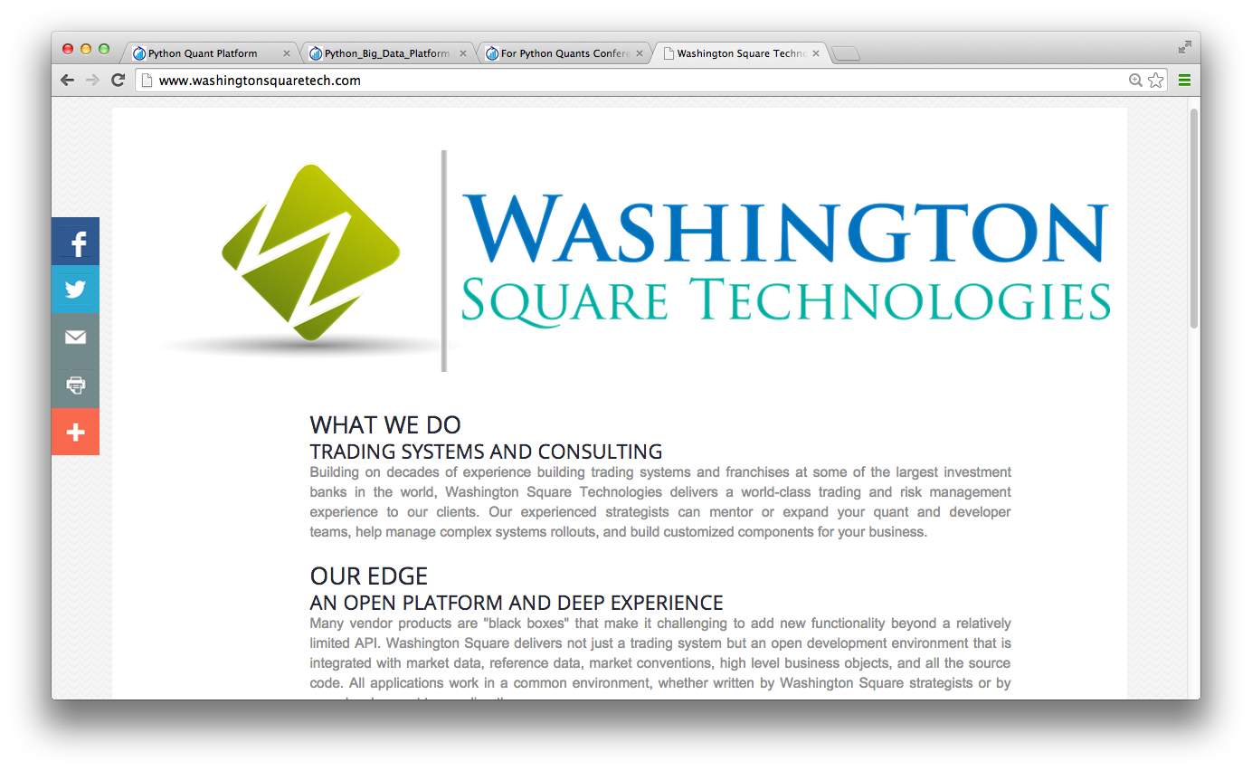
Example: Washington Square Technologies¶

Trading and Risk Management powered by Python.

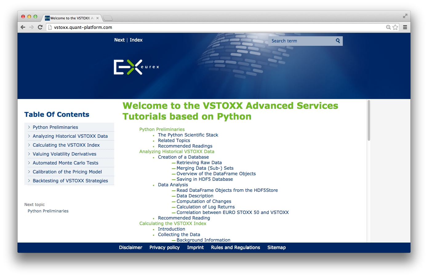
Example: Eurex Advanced Services (VSTOXX & Variance Futures)¶

Python-based tutorials by Eurex (http://www.eurexchange.com/vstoxx/).

Books¶

By others:

Python for Financial Modelling @ Wiley Finance (2009)
Python for Finance @ Packt Publishing (2014)
Mastering Python for Finance @ Packt Publishing (2015)
Mastering pandas for Finance @ Packt Publishing (2015)
SABR and SABR LIBOR Market Models in Practice @ Palgrave Macmillan (2015)
...

By myself:

Python for Finance – Analyze Big Financial Data @ O'Reilly (2014)
Derivatives Analytics with Python @ Wiley Finance (2015)
Listed Volatility and Variance Derivatives — A Python-based Guide @ Wiley Finance (2016)

Published in December 2014.

Published in July 2015.

Forthcoming in 2016.

Financial Research¶

"The appendices present an implementation in Python of our experiments." (p. 3)

Education¶

Master of Financial Engineering @ Baruch College CUNY
Numerical Option Pricing with Python @ Saarland University
Python-based Lectures at CQF Program @ Fitch Learning
Python for Finance Certification @ Fitch Learning
...

Baruch College Web site:

"Knowledge and Skills: Our graduates have working experience with C++, VBA, Python, R, and Matlab for financial applications. They share an exceptionally strong work ethic and possess excellent interpersonal, teamwork, and communication skills."

Training¶

By others:

Python for Finance @ Continuum Analytics
Python for Finance @ Enthought

By myself:

Python for Quant Finance @ Python for Quant Finance Meetup Group
Python for Finance @ http://quantshub.com
Introductory, Technical & Financial Python Workshops @ CQF Institute/Fitch Learnings
...

In [35]:

HTML('<iframe src=http://quantshub.com/content/python-finance-yves-j-hilpisch \
        width=100% height=550></iframe>')

Out[35]:

Meetups¶

Python for Quant Finance London (1,050 members)
Python for Quant Finance NYC
Python Big Data Analytics Berlin
...

For Python Quants Conference¶

1st conference in New York City on 14. March 2014
2nd conference in London on 28. November 2014
3rd conference in New York City on 01. May 2015
4th conference in London on 27. November 2015

http://fpq.io

In [36]:

HTML('<iframe src="http://fpq.io" \
     width=100% height=650></iframe>')

Out[36]:

Python – MMA of the Technology World

My wish for Python in the future: to become THE glue language and platform in Quant Finance for

data analytics
financial analytics
development efforts in general
performance technologies
unifying processes from exploration to production
...

Python has the potential to accomplish what MMA has done for the Martial Arts.

Disclaimer¶

Do not use Python at your own risk.¶

Contact us¶

Please contact us if you have any questions or want to get involved in our Python community events.

The Python Quants

tpq.io | @dyjh

team@tpq.io

Python Quant Platform | http://quant-platform.com

Derivatives Analytics with Python | Derivatives Analytics @ Wiley Finance

Python for Finance | Python for Finance @ O'Reilly