![]()
Performance Python
For Numerical Algorithms
Dr. Yves J. Hilpisch
The Python Quants GmbH
Berlin, EuroPython Conference 2014
About Us
The Python Quant
- Founder and Managing Partner of The Python Quants GmbH
- Lecturer Mathematical Finance at Saarland University
- Co-organizer of "For Python Quants" conference in New York
- Organizer of "Python for Quant Finance" meetup in London
- Organizer of "Python for Big Data Analytics" meetup in Berlin
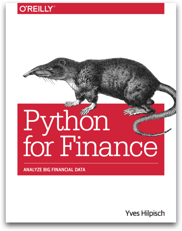
- Book (2014) "Python for Finance", O'Reilly
- Book (2015) "Derivatives Analytics with Python", Wiley Finance
- Dr.rer.pol in Mathematical Finance
- Graduate in Business Administration
- Martial Arts Practitioner and Fan
See www.hilpisch.com.
On 13th of October 2014, a online training course based on the book – also covering Performance Python – will go live on the Quantshub.com platform.
from IPython.display import HTML
HTML('<iframe src=http://quantshub.com/content/python-finance-yves-j-hilpisch width=900 height=450></iframe>')
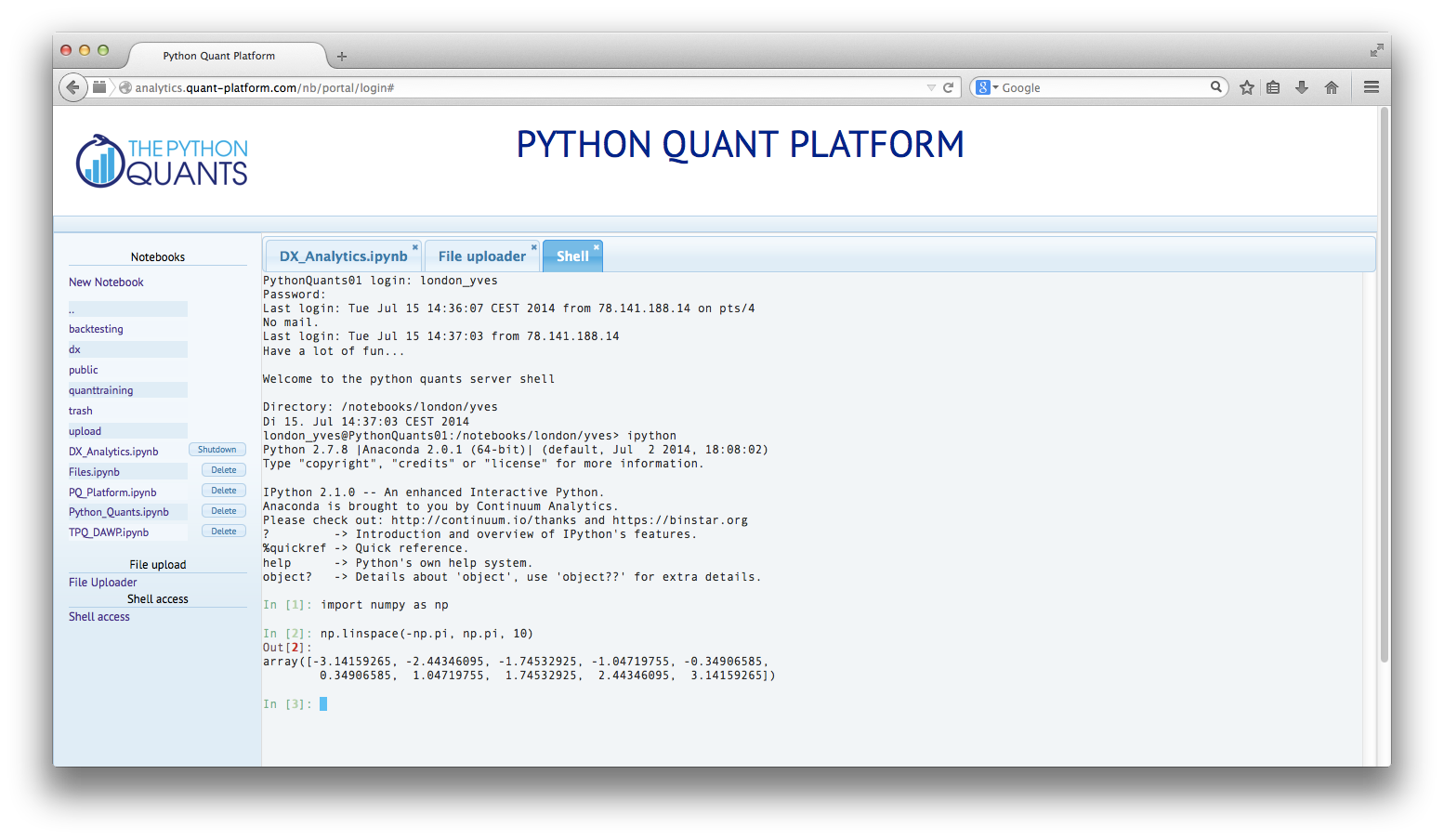
Currently we are mainly working on the Python Quant Platform (cf. http://quants-platform.com) – a Web-based financial analytics platform for Quants, with collaboration features and our analytics suite DEXISION as well as the financial analytics library DX Analytics.
IPython Notebook
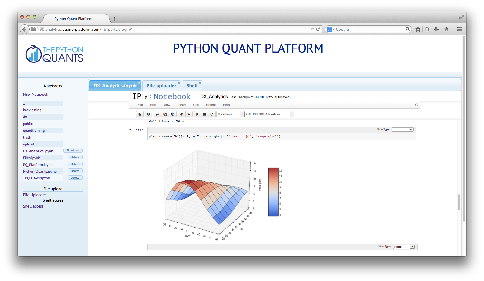 |
IPython Shell
 |
|---|---|
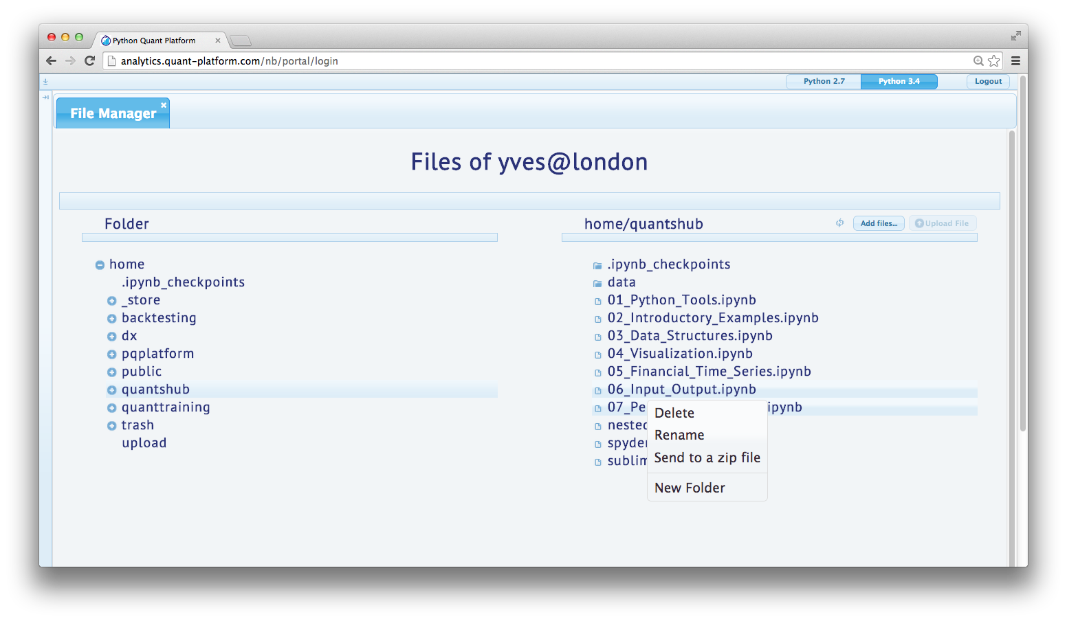
Easy File Management
 |
Vim Editing via Shell
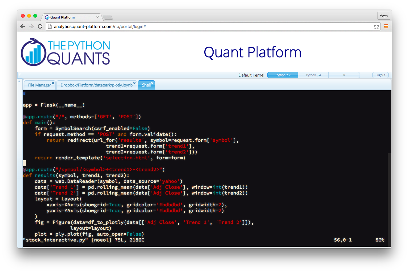 |
What this Talks is about
When it comes to performance critical applications two things should always be checked: are we using the right implementation paradigm and are we using the right performance libraries?
In addition to considering different implementation paradigms, this talk introduces the following performance libraries:
- Cython
- IPython.Parallel
- multiprocessing
- numexpr
- Numba
- NumbaPro
Python Paradigms and Performance
A function we use regularly to compare performance.
def perf_comp_data(func_list, data_list, rep=3, number=1):
    ''' Function to compare the performance of different functions.

    Parameters
    ==========
    func_list : list
        list with function names as strings
    data_list : list
        list with data set names as strings
    rep : int
        number of repetitions of the whole comparison
    number : int
        number of executions for every function
    '''
    from timeit import repeat
    res_list = {}
    for name in enumerate(func_list):
        stmt = name[1] + '(' + data_list[name[0]] + ')'
        setup = "from __main__ import " + name[1] + ', ' \
                                    + data_list[name[0]]
        results = repeat(stmt=stmt, setup=setup,
                         repeat=rep, number=number)
        res_list[name[1]] = sum(results) / rep
    res_sort = sorted(res_list.iteritems(),
                      key=lambda (k, v): (v, k))
    for item in res_sort:
        rel = item[1] / res_sort[0][1]
        print 'function: ' + item[0] + \
              ', av. time sec: %12.8f, ' % item[1] \
            + 'relative: %9.1f' % rel
In finance, like in other scientific and data-intensive disciplines, numerical computations on large data sets can be quite time consuming. Consider the following mathematical expression.
$$ \begin{equation} y = \sqrt{|\cos(x)|} + \sin(2 + 3x) \end{equation} $$
This is easily translated into a Python function.
from math import *
def f(x):
    return abs(cos(x)) ** 0.5 + sin(2 + 3 * x)
Using the range function we can generate efficiently a list object with 500,000 numbers which we can work with.
I = 500000
a_py = range(I)
Consider now different implementations (1).
def f1(a):
    res = []
    for x in a:
        res.append(f(x))
    return res
Consider now different implementations (2).
def f2(a):
    return [f(x) for x in a]
Consider now different implementations (3).
def f3(a):
    ex = 'abs(cos(x)) ** 0.5 + sin(2 + 3 * x)'
    return [eval(ex) for x in a]
Consider now different implementations (4).
import numpy as np
a_np = np.arange(I)
def f4(a):
    return (np.abs(np.cos(a)) ** 0.5 +
            np.sin(2 + 3 * a))
Consider now different implementations (5).
import numexpr as ne
def f5(a):
    ex = 'abs(cos(a)) ** 0.5 + sin(2 + 3 * a)'
    ne.set_num_threads(1)
    return ne.evaluate(ex)
Consider now different implementations (6).
def f6(a):
    ex = 'abs(cos(a)) ** 0.5 + sin(2 + 3 * a)'
    ne.set_num_threads(4)
    return ne.evaluate(ex)
In total, the same task, i.e. the evaluation of the numerical expression on an array of size 500,000, is implemented in six different ways:
- standard Python function with explicit looping
- list comprehension approach with implicit looping
- list comprehension approach with implicit looping and using
eval NumPyvectorized implementation- single-threaded implementation using
numexpr - multi-threaded implementation using
numexpr
Let us compare the performance.
func_list = ['f1', 'f2', 'f3', 'f4', 'f5', 'f6']
data_list = ['a_py', 'a_py', 'a_py', 'a_np', 'a_np', 'a_np']
perf_comp_data(func_list, data_list, rep=1)
Memory Layout and Performance
A subtle but sometimes important topic is memory layout with NumPy arrays.
import numpy as np
np.zeros((3, 3), dtype=np.float64, order='C')
  # C layout
Consider the C-like, i.e. row-wise, storage.
c = np.array([[ 1.,  1.,  1.],
              [ 2.,  2.,  2.],
              [ 3.,  3.,  3.]], order='C')
In this case, the 1s, the 2s and the 3s are stored next to each other.
By contrast, consider the Fortran-like, i.e. column-wise, storage.
f = np.array([[ 1.,  1.,  1.],
              [ 2.,  2.,  2.],
              [ 3.,  3.,  3.]], order='F')
Now, the data is stored in a way that 1, 2, 3 are next to each other for each column.
Let's see whether the memory layout makes a difference in some way when the array is large.
x = np.random.standard_normal((3, 1500000))
C = np.array(x, order='C')
F = np.array(x, order='F')
x = 0.0
First, calculating sums with C order.
%timeit C.sum(axis=0)
%timeit C.sum(axis=1)
Second, standard deviations with C order.
%timeit C.std(axis=0)
%timeit C.std(axis=1)
Third, sums with F order.
%timeit F.sum(axis=0)
%timeit F.sum(axis=1)
Fourth, standard deviations with F order.
%timeit F.std(axis=0)
%timeit F.std(axis=1)
Parallel Computing
A tool for parallel computing with Python is the IPython.parallel library. Another one is the multiprocessing module of Python itself. As an example, we take a Monte Carlo algorithm for the Black-Scholes-Merton (1973) model with the SDE:
$$ \begin{equation} dS_t = r S_t dt + \sigma S_t dZ_t \end{equation} $$
We simulate this model (as in part 2) and calculate the Monte Carlo estimator for a European call option:
$$ \begin{equation} C_0 = e^{-rT} \frac{1}{I} \sum_I \max(S_T(i) - K, 0) \end{equation} $$
The Implementation of the Algorithm
A function implementing the Monte Carlo valuation for the Black-Scholes-Merton set-up could look like follows:
def bsm_mcs_valuation(strike):
    import numpy as np
    S0 = 100.; T = 1.0; r = 0.05; vola = 0.2
    M = 50; I = 20000
    dt = T / M
    rand = np.random.standard_normal((M + 1, I))
    S = np.zeros((M + 1, I)); S[0] = S0
    for t in range(1, M + 1):
        S[t] = S[t-1] * np.exp((r - 0.5 * vola ** 2) * dt
                               + vola * np.sqrt(dt) * rand[t])
    value = (np.exp(-r * T)
                     * np.sum(np.maximum(S[-1] - strike, 0)) / I)
    return value
The Sequential Calculation
As the benchmark case we take the sequential valuation of 100 options with different strike prices.
def seq_value(n):
    strikes = np.linspace(80, 120, n)
    option_values = []
    for strike in strikes:
        option_values.append(bsm_mcs_valuation(strike))
    return strikes, option_values
n = 100  # number of options to be valued
%time strikes, option_values_seq = seq_value(n)
The results visualized.
import matplotlib.pyplot as plt
%matplotlib inline
plt.figure(figsize=(8, 4))
plt.plot(strikes, option_values_seq, 'b')
plt.plot(strikes, option_values_seq, 'r.')
plt.grid(True)
plt.xlabel('strikes')
plt.ylabel('European call option values')

The Parallel Calculation
IPython.parallel needs the information which cluster to use for the parallel execution of code (local, remote, etc.). You can, for example, simply start a local cluster (eg via the IPython Notebook Dashboard).
from IPython.parallel import Client
c = Client(profile="default")
view = c.load_balanced_view()
The function implementing the parallel valuation.
def par_value(n):
    strikes = np.linspace(80, 120, n)
    option_values = []
    for strike in strikes:
        value = view.apply_async(bsm_mcs_valuation, strike)
        option_values.append(value)
    c.wait(option_values)
    return strikes, option_values
And the parallel execution.
%time strikes, option_values_obj = par_value(n)
The parallel execution does not return option values directly, it rather returns more complex results objects.
option_values_obj[0].metadata
The valuation result itself is stored in the result attribute of the object.
option_values_obj[0].result
The complete results list.
option_values_par = []
for res in option_values_obj:
    option_values_par.append(res.result)
And the respective plot.
plt.figure(figsize=(8, 4))
plt.plot(strikes, option_values_seq, 'b', label='Sequential')
plt.plot(strikes, option_values_par, 'r.', label='Parallel')
plt.grid(True); plt.legend(loc=0)
plt.xlabel('strikes')
plt.ylabel('European call option values')

Performance Comparison
Let us compare the performance a bit more rigorously.
n = 25  # number of option valuations
func_list = ['seq_value', 'par_value']
data_list = 2 * ['n']
perf_comp_data(func_list, data_list, rep=3)
Multiprocessing
IPython.parallel scales over small and medium-sized clusters (e.g. with 256 nodes). Sometimes it is, however, helpful to parallelize code execution locally. Here, the multiprocessing module of Python might prove beneficial.
import multiprocessing as mp
Consider the following function to simulate a geometric Brownian motion.
import math
def simulate_geometric_brownian_motion(p):
    M, I = p
      # time steps, paths
    S0 = 100; r = 0.05; sigma = 0.2; T = 1.0
      # model parameters
    dt = T / M
    paths = np.zeros((M + 1, I))
    paths[0] = S0
    for t in range(1, M + 1):
        paths[t] = paths[t - 1] * np.exp((r - 0.5 * sigma ** 2) * dt +
                    sigma * math.sqrt(dt) * np.random.standard_normal(I))
    return paths
This function returns simulated paths given the parametrization for M and I.
paths = simulate_geometric_brownian_motion((5, 2))
paths
Let us implement a test series on notebook with 4 cores and the following parameter values.
I = 10000  # number of paths
M = 10  # number of time steps
t = 32  # number of tasks/simulations
# running on machine with 4 cores/8 threads
from time import time
times = []
for w in range(1, 9):
    t0 = time()
    pool = mp.Pool(processes=w)
      # the pool of workers
    result = pool.map(simulate_geometric_brownian_motion, t * [(M, I), ])
      # the mapping of the function to the list of parameter tuples
    times.append(time() - t0)
Performance scales linearly with the number of cores used.
plt.plot(range(1, 9), times)
plt.plot(range(1, 9), times, 'ro')
plt.grid(True)
plt.xlabel('number of processes')
plt.ylabel('time in seconds')
plt.title('%d Monte Carlo simulations' % t)

Dynamic Compiling
Numba is an open source, NumPy-aware optimizing compiler for Python code. Cf. http://numba.pydata.org.
It uses the LLVM compiler infrastructure. Cf. http://www.llvm.org.
Introductory Example
Let us start with a problem that typically leads to performance issues in Python: alogrithms with nested loops.
from math import cos, log
def f_py(I, J):
    res = 0
    for i in range(I):
        for j in range (J):
            res += int(cos(log(1)))
    return res
I, J = 5000, 5000
%time f_py(I, J)
In principle, this can be vectorized with the help of NumPy ndarray objects.
import numpy as np
def f_np(I, J):
    a = np.ones((I, J), dtype=np.float64)
    return int(np.sum(np.cos(np.log(a)))), a
%time res, a = f_np(I, J)
However, the ndarray object consumes 200 MB of memory.
a.nbytes
Consider therefore the Numba alternative.
import numba as nb
f_nb = nb.jit(f_py)
The new function can be called directly from Python. At the first time, with a "huge" overhead.
%time res = f_nb(I, J)
%time res = f_nb(I, J)
res
Let us compare the performance of the different alternatives more systematically.
func_list = ['f_py', 'f_np', 'f_nb']
data_list = 3 * ['I, J']
perf_comp_data(func_list, data_list, rep=1)
Binomial Option Pricing
Consider a parametrization for the binomial option pricing model of Cox-Ross-Rubinstein (1979) as follows.
from math import sqrt, exp
# model & option Parameters
S0 = 100.  # initial index level
T = 1.  # call option maturity
r = 0.05  # constant short rate
vola = 0.20  # constant volatility factor of diffusion

# time parameters
M = 1000  # time steps
dt = T / M  # length of time interval
df = exp(-r * dt)  # discount factor per time interval

# binomial parameters
u = exp(vola * sqrt(dt))  # up-movement
d = 1 / u  # down-movement
q = (exp(r * dt) - d) / (u - d)  # martingale probability
An implementation of the binomial algorithm for European options consists mainly of these parts:
- index level simulation
- inner value calculation
- risk-neutral discounting
In Python this might take on the form (using NumPy arrays).
import numpy as np
def binomial_py(strike):
    # LOOP 1 - Index Levels
    S = np.zeros((M + 1, M + 1), dtype=np.float64)
      # index level array
    S[0, 0] = S0
    z1 = 0
    for j in xrange(1, M + 1, 1):
        z1 = z1 + 1
        for i in xrange(z1 + 1):
            S[i, j] = S[0, 0] * (u ** j) * (d ** (i * 2))

    # LOOP 2 - Inner Values
    iv = np.zeros((M + 1, M + 1), dtype=np.float64)
      # inner value array
    z2 = 0
    for j in xrange(0, M + 1, 1):
        for i in xrange(z2 + 1):
            iv[i, j] = max(S[i, j] - strike, 0)
        z2 = z2 + 1

    # LOOP 3 - Valuation
    pv = np.zeros((M + 1, M + 1), dtype=np.float64)
      # present value array
    pv[:, M] = iv[:, M]  # initialize last time point
    z3 = M + 1
    for j in xrange(M - 1, -1, -1):
        z3 = z3 - 1
        for i in xrange(z3):
            pv[i, j] = (q * pv[i, j + 1] +
                        (1 - q) * pv[i + 1, j + 1]) * df
    return pv[0, 0]
This function returns the present value of a European call option with parameters as specified before.
%time round(binomial_py(100), 3)
We can compare this result with the estimated value the Monte Carlo function bsm_mcs_valuation returns.
%time round(bsm_mcs_valuation(100), 3)
First improvement: NumPy vectorization.
def binomial_np(strike):
    # Index Levels with NumPy
    mu = np.arange(M + 1)
    mu = np.resize(mu, (M + 1, M + 1))
    md = np.transpose(mu)
    mu = u ** (mu - md)
    md = d ** md
    S = S0 * mu * md

    # Valuation Loop
    pv = np.maximum(S - strike, 0)
    qu = np.zeros((M + 1, M + 1), dtype=np.float64)
    qu[:, :] = q
    qd = 1 - qu
    z = 0
    for t in range(M - 1, -1, -1):  # backwards iteration
        pv[0:M - z, t] = (qu[0:M - z, t] * pv[0:M - z, t + 1]
                        + qd[0:M - z, t] * pv[1:M - z + 1, t + 1]) * df
        z += 1
    return pv[0, 0]
Check the performance of the NumPy version.
M = 1000  # reset number of time steps
%time round(binomial_np(100), 3)
Let us try the Numba dynamic compiling approach (remember the overhead of the first call).
binomial_nb = nb.jit(binomial_py)
%time round(binomial_nb(100), 3)
%time round(binomial_nb(100), 3)
A rigorous performance comparison.
func_list = ['binomial_py', 'binomial_np', 'binomial_nb']
K = 100.
data_list = 3 * ['K']
perf_comp_data(func_list, data_list, rep=1)
In summary, we can state the following:
- efficiency: using
Numbainvolves only little additional effort - speed-up:
Numbaleads often to significant improvements of execution speed, even compared to vectorizedNumPyimplementations - memory: with
Numbathere is no need to initialize large array objects; the compiler specializes the machine code to the problem at hand and maintains memory efficiency
Static Compiling with Cython
Cython is a static compiler for (annotated) Python code. In effect, Cython represents a hybrid language between Python and C as the name already suggests.
Again, a simple example function with a nested loop.
def f_py(I, J):
    res = 0.  # we work on a float object
    for i in range(I):
        for j in range (J * I):
            res += 1
    return res
I, J = 500, 500
%time f_py(I, J)
Consider now the Cython file with the static type declarations (and note the suffic .pyx)
%loadpy nested_loop.pyx
#
# Nested loop example with Cython
# nested_loop.pyx
#
def f_cy(int I, int J):
    cdef double res = 0
    # double float much slower than int or long
    for i in range(I):
        for j in range (J * I):
            res += 1
    return res
When no special C modules are needed, there is an easy way to import such a module, namely via pyximport.
import pyximport
pyximport.install()
This allows us now to directly import from the Cython module.
from nested_loop import f_cy
Now, we can check the performance of the Cython function.
%time res = f_cy(I, J)
res
When working in IPython Notebook there is a more convenient way to use Cython: cythonmagic.
%load_ext cythonmagic
%%cython
#
# Nested loop example with Cython
#
def f_cy(int I, int J):
    cdef double res = 0
    # double float much slower than int or long
    for i in range(I):
        for j in range (J * I):
            res += 1
    return res
%time res = f_cy(I, J)
res
Let us return Numba.
import numba as nb
f_nb = nb.jit(f_py)
res = f_nb(I, J)
res
%timeit f_nb(I, J)
Finally, again the more rigorous comparison.
func_list = ['f_py', 'f_cy', 'f_nb']
I, J = 500, 500
data_list = 3 * ['I, J']
perf_comp_data(func_list, data_list, rep=1)
Generation of Random Numbers on GPUs
The last topic in this chapter is the use of devices for massively parallel operaitions, i.e. General Purpose Graphical Processing Units (GPGPUs or simply GPUs). To use a Nvidia GPU, we need to have CUDA (Compute Unified Device Architecture, cf. http://en.wikipedia.org/wiki/CUDA) installed.
An easy way to harness the power of Nvidia GPUs is the use of NumbaPro, a performance library by Continuum Analytics that dynamically compiles Python code for the GPU (or a multi-core CPU) – similar to Numba.
We use the GPU to generate pseudo-randum numbers.
from numbapro.cudalib import curand
As the benchmark case, we define a function using NumPy to generate pseudo-random numbers.
def get_randoms(x, y):
    rand = np.random.standard_normal((x, y))
    return rand
get_randoms(2, 2)
Now the function for the Nvidia GPU.
def get_cuda_randoms(x, y):
    rand = np.empty((x * y), np.float64)
        # rand serves as a container for the randoms,
        # CUDA only fills 1-D arrays
    prng = curand.PRNG(rndtype=curand.PRNG.XORWOW)
        # the argument sets the random number algorithm
    prng.normal(rand, 0, 1)  # filling the container
    rand = rand.reshape((x, y))
        # to be 'fair', we reshape rand to 2 dimensions
    return rand
get_cuda_randoms(2, 2)
A first comparison of the performance.
%timeit a = get_randoms(1000, 1000)
%timeit a = get_cuda_randoms(1000, 1000)
Now a more systematic routine to compare the performance.
import time as t
step = 1000
def time_comparsion(factor):
    cuda_times = list()
    cpu_times = list()
    for j in range(1, 10002, step):
        i = j * factor
        t0 = t.time()
        a = get_randoms(i, 1)
        t1 = t.time()
        cpu_times.append(t1 - t0)
        t2 = t.time()
        a = get_cuda_randoms(i, 1)
        t3 = t.time()
        cuda_times.append(t3 - t2)
    print "Bytes of largest array %i" % a.nbytes
    return cuda_times, cpu_times
And a helper function to visualize performance results.
def plot_results(cpu_times, cuda_times, factor):
    plt.plot(x * factor, cpu_times,'b', label='NUMPY')
    plt.plot(x * factor, cuda_times, 'r', label='CUDA')
    plt.legend(loc=0)
    plt.grid(True)
    plt.xlabel('size of random number array')
    plt.ylabel('time')
    plt.axis('tight')
The first test series with a medium workload.
factor = 100
cuda_times, cpu_times = time_comparsion(factor)
x = np.arange(1, 10002, step)
plot_results(cpu_times, cuda_times, factor)

The second test series with a pretty low workload.
factor = 10
cuda_times, cpu_times = time_comparsion(factor)
plot_results(cpu_times, cuda_times, factor)

Third test series with more heavy workloads. The largest random number array is 400 MB in size.
%%time
factor = 5000
cuda_times, cpu_times = time_comparsion(factor)
plot_results(cpu_times, cuda_times, factor)

Hardware-Bound I/O Operations
Chapter 8 of my Python for Finance book covers hardware-bound I/O with Python.
With Python it is pretty efficient to reach I/O speeds only limited by the hardware that is used. Consider a larger NumPy ndarray object.
import numpy as np
%time a = np.random.standard_normal((10000, 10000))
a.nbytes
Writing and reading such a NumPy ndarray object "natively" to HDD/SDD is typically done at the speed that the hardware allows.
%time np.save('a_on_disk', a)
ll a_*
%time b = np.load('a_on_disk.npy')
Making sure we got indeed the same data and deleting all objects.
%time np.allclose(a, b)
del a; del b
!rm a_on_disk.npy
![]()
www.hilpisch.com | www.pythonquants.com
Python for Finance – my O'Reilly book
Derivatives Analytics with Python – forthcoming at Wiley Finance